Meta Analysis 01: Clinical multi center study

We follow the following publication:

Ding-Geng (Din) Chen, Karl E. Peace (2013): Applied Meta-Analysis with R. CRC Press, Taylor & Francis Group, Boca Raton (FL), 321pp. ISBN-10: 1466505990, ISBN-13: 978-1466505995. See also here

The applications in this publication are programmed in R. We do it in Python here. We will describe the cases in a minimalistic way only. For details consult the book please.

The case

The example in chapter 1 mimics a multi center study of a diastolic blood pressure decreasing drug. The data are generated by ading random noise to a normal distribution. The generated data are concatenated to a data framework which allows for queries, statistical analysis and graphical displays. As a result we get a running workflow for a typical type of analysis.

The example generates for each of the 5 clinical centers the data series for the control group and for the treated group. A series includes the variables age, base pressure, endpoint pressure, difference between them, the number of the clinical center and the type of treament ('drug' = yes, 'ctrl' = no)

Implementation with Python

Import the Python librarys

The add-on libraries to the core of Python are NumPy for the matrix/array data types, and Pandas for data structures and prelimnary data analysis. The statistical package StatsModels is used for the regression model and the analysis of variances. Seaborn is used for the grafics which is based on Matplotlib

import numpy  as np
import pandas as pd
import statsmodels.api as sm
import statsmodels.formula.api as smf
import seaborn as sns
sns.set(style="ticks")
%matplotlib inline

Define the functions to generate the data

The first 2 moments - mean and sdev - are used as input to generate a normal distributed data series.

def generateData(nobs,center,treatment,bp_μ, bp_σ,bp_δμ, age_μ, age_σ):
                # nobs = n observations     
                # bp_μ = blood pressure mean
                # bp_σ = blood pressure sdev
                # bp_δμ= mean change of blood pressure due to drug; = 0 for no drug
                # bp_Δ = difference between endpoint and baseline of the clinical trial
    bp_base = np.random.normal(bp_μ        , bp_σ, nobs)   # random normal
    bp_end  = np.random.normal(bp_μ - bp_δμ, bp_σ, nobs)   # random normal
    bp_Δ    = bp_end - bp_base

    age     = np.random.normal(age_μ, age_σ, nobs)  # age, random normal
    cen     = center*np.ones_like(age,dtype=np.int) # number of the clinical center
    trt     = [treatment for t in range(nobs)]      # treatment: with drug or ctrl
    index   = np.arange(nobs)                       # data index

    myDataStack = {'bp_base': bp_base,'bp_end':bp_end, 'bp_Δ':bp_Δ,
                   'age':age,'cen':cen,'trt':trt}
    return pd.DataFrame(myDataStack,index=index)

Set the input data

In this example it is assumed that 5 clinical centers are involved in the multi center study and that bp_δμ (change of mean blood pressure) is the only parameter that varies between the centers. For the control group bp_δμ_ctrl = 0

#------ main --------------------------------
#---- data we keep constant in this example:
nObs=100;  # n observations 
trt_ctrl   = 'ctrl'  # control group
trt_drug   = 'drug'  # group with treatment
bp_δμ_ctrl = 0       # change of mean blood pressure in the ctrl-group
bp_μ  = 100          # mean blood pressure
bp_σ  = 10           # sdev blood pressure
age_μ = 50           # mean age
age_σ = 10           # sdev age
#----- data we change to build the series
center1 = 1;  bp_δμ_1 = 10   # clinical center; mean treatment effect 
center2 = 2;  bp_δμ_2 = 13
center3 = 3;  bp_δμ_3 = 15
center4 = 4;  bp_δμ_4 =  8
center5 = 5;  bp_δμ_5 = 10

Now generate the data series and build a DataFrame

Each clinical center has a data series of the same length for the control group and the treated group. All data are concatenated into 1 data frame.

# series 1
dat4ctrl = generateData(nObs,center1,trt_ctrl,bp_μ,bp_σ,bp_δμ_ctrl,age_μ, age_σ)
dat4drug = generateData(nObs,center1,trt_drug,bp_μ,bp_σ,bp_δμ_1   ,age_μ, age_σ)
d1 = pd.concat([dat4ctrl,dat4drug],ignore_index=True)
# series 2
dat4ctrl = generateData(nObs,center2,trt_ctrl,bp_μ,bp_σ,bp_δμ_ctrl,age_μ, age_σ)
dat4drug = generateData(nObs,center2,trt_drug,bp_μ,bp_σ,bp_δμ_2   ,age_μ, age_σ)
d2 = pd.concat([dat4ctrl,dat4drug],ignore_index=True)
# series 3
dat4ctrl = generateData(nObs,center3,trt_ctrl,bp_μ,bp_σ,bp_δμ_ctrl,age_μ, age_σ)
dat4drug = generateData(nObs,center3,trt_drug,bp_μ,bp_σ,bp_δμ_3   ,age_μ, age_σ)
d3 = pd.concat([dat4ctrl,dat4drug],ignore_index=True)
# series 4
dat4ctrl = generateData(nObs,center4,trt_ctrl,bp_μ,bp_σ,bp_δμ_ctrl,age_μ, age_σ)
dat4drug = generateData(nObs,center4,trt_drug,bp_μ,bp_σ,bp_δμ_4   ,age_μ, age_σ)
d4 = pd.concat([dat4ctrl,dat4drug],ignore_index=True)
# series 5
dat4ctrl = generateData(nObs,center5,trt_ctrl,bp_μ,bp_σ,bp_δμ_ctrl,age_μ, age_σ)
dat4drug = generateData(nObs,center5,trt_drug,bp_μ,bp_σ,bp_δμ_5   ,age_μ, age_σ)
d5 = pd.concat([dat4ctrl,dat4drug],ignore_index=True)
# build 1 DataFrame with all data
dAll = pd.concat([d1,d2,d3,d4,d5],ignore_index=True)

Let's have a look at the head of the first few lines of the data frame:

dAll.head(5)

	age	bp_base	bp_end	bp_Δ	cen	trt
0	60.720858	111.664456	99.437909	-12.226547	1	ctrl
1	36.035688	89.109796	88.445715	-0.664080	1	ctrl
2	38.823806	92.925221	97.549218	4.623998	1	ctrl
3	38.783952	91.520139	104.185235	12.665097	1	ctrl
4	65.327808	93.283620	104.308016	11.024396	1	ctrl

Print the statistics of the data

dAll.groupby(['cen', 'trt']).agg(['count','mean','std'])

		age			bp_base			bp_end			bp_Δ
		count	mean	std	count	mean	std	count	mean	std	count	mean	std
cen	trt
1	ctrl	100	48.467260	10.194531	100	98.567163	11.792550	100	99.793300	9.211106	100	1.226136	13.389781
1	drug	100	49.628733	9.628830	100	99.935044	10.373236	100	87.838175	9.571521	100	-12.096870	14.092291
2	ctrl	100	49.215135	10.550840	100	98.480676	10.410645	100	99.435871	10.324950	100	0.955195	14.974590
2	drug	100	50.154245	10.313113	100	98.144471	9.870396	100	86.472468	10.531072	100	-11.672004	14.280153
3	ctrl	100	47.850356	9.693100	100	99.867286	9.946296	100	99.712728	9.894162	100	-0.154558	14.311047
3	drug	100	49.427241	10.435070	100	98.287170	10.428239	100	86.059913	10.143901	100	-12.227257	14.219824
4	ctrl	100	48.263132	9.648512	100	99.514863	9.863520	100	99.043574	9.933129	100	-0.471289	13.328751
4	drug	100	49.930536	10.266096	100	99.877485	10.086439	100	91.581340	9.771715	100	-8.296145	13.936570
5	ctrl	100	50.424546	9.768934	100	99.979968	10.454416	100	100.016502	10.191461	100	0.036535	14.902816
5	drug	100	49.665251	10.003291	100	98.986446	9.906621	100	90.535263	9.178024	100	-8.451183	13.524656

Play around with the different types of plots

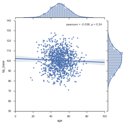
This first plot contains all data, age vs base blood pressure, treated and untreated over all 5 clinical centers. On the east and the north side of the graph you should recognize the generated normal distributions in the bar plots, whereas the plotted lines are nice looking splines over the bar data only. The plotted line in the graph with y = base blood pressure should be horizontal most of the time and have a value of about 100 beceause this the mean given as input.

Each data series has 100 observations, so 1'000 data points are included in this graph.

sns.jointplot(x="age", y="bp_base", data= dAll, kind="reg");

png

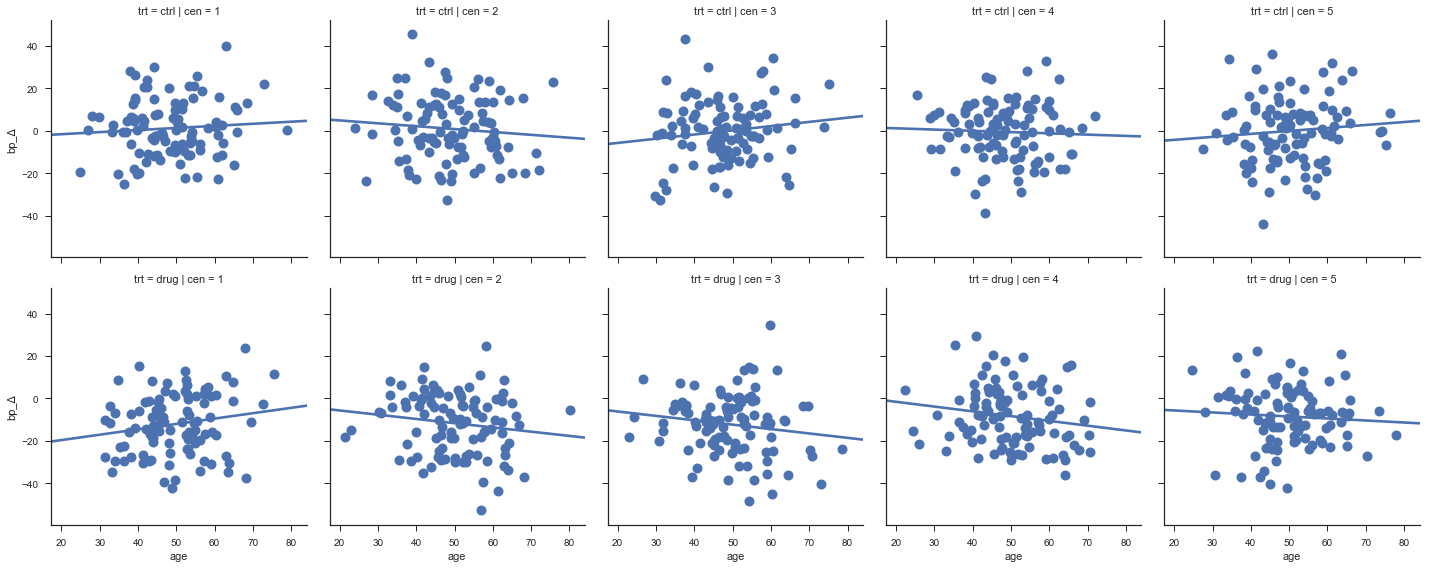
The next graph displays the change of blood pressure vs age for each center. The change of blood pressure should be more negative for the treated groups than for the control group hopefully, beceause this corresponds to the mean given as input.

sns.lmplot(x="age", y="bp_Δ", col="cen", row="trt", data=dAll,
           ci=None, palette="muted", size=4,
           scatter_kws={"s": 100, "alpha": 1 });

png

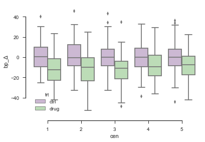
The change of blood pressure, displayed for the ctrl-group and the trt-group for each clinical center, is summarized in a box plot.

sns.boxplot(x="cen", y="bp_Δ", hue="trt", data=dAll, palette="PRGn")
sns.despine(offset=10, trim=True)

png

Data analysis of each center

With these preliminary graphical illustrations, we now proceed to data analysis. We start with the individual center effects. We subset the data from each center to perform an analysis of variance. We consider a treament effect as statistically significant at p-value $<0.05$ e.g.

e_c1 = smf.ols(formula='bp_Δ ~ trt', data = dAll[dAll["cen"]==1]).fit()
t_c1 = sm.stats.anova_lm(e_c1, typ=1)
print('Center = 1'); print(t_c1, '\n')

e_c2 = smf.ols(formula='bp_Δ ~ trt', data = dAll[dAll["cen"]==2]).fit()
t_c2 = sm.stats.anova_lm(e_c2, typ=1)
print("Center = 2");  print(t_c2, '\n')

e_c3 = smf.ols(formula='bp_Δ ~ trt', data = dAll[dAll["cen"]==3]).fit()
t_c3 = sm.stats.anova_lm(e_c3, typ=1)
print("Center = 3");  print(t_c3, '\n')

e_c4 = smf.ols(formula='bp_Δ ~ trt', data = dAll[dAll["cen"]==4]).fit()
t_c4 = sm.stats.anova_lm(e_c4, typ=1)
print("Center = 4");  print(t_c4, '\n')

e_c5 = smf.ols(formula='bp_Δ ~ trt', data = dAll[dAll["cen"]==5]).fit()
t_c5 = sm.stats.anova_lm(e_c5, typ=1)
print("Center = 5");  print(t_c5, '\n')

Center = 1
             df        sum_sq      mean_sq         F        PR(>F)
trt         1.0   8875.124407  8875.124407  46.97338  8.913676e-11
Residual  198.0  37410.010029   188.939445       NaN           NaN

Center = 2
             df        sum_sq      mean_sq          F        PR(>F)
trt         1.0   7972.307055  7972.307055  37.239755  5.404231e-09
Residual  198.0  42387.948440   214.080548        NaN           NaN

Center = 3
             df        sum_sq      mean_sq          F        PR(>F)
trt         1.0   7287.503584  7287.503584  35.809995  1.003735e-08
Residual  198.0  40293.937324   203.504734        NaN           NaN

Center = 4
             df        sum_sq      mean_sq          F    PR(>F)
trt         1.0   3061.418522  3061.418522  16.464392  0.000071
Residual  198.0  36816.473763   185.941787        NaN       NaN

Center = 5
             df        sum_sq      mean_sq          F    PR(>F)
trt         1.0   3602.067373  3602.067373  17.787537  0.000038
Residual  198.0  40096.015373   202.505128        NaN       NaN

Data Analysis with pooled data from five centers

Remember data generation: Different treatment effects has been assigned to the different clinical centers but treatment has not been related to age. We hope to recognize that in the analysis again of course. We start to fit a model for the blood pressure difference bp_Δ with 3-way interactions among treatment, center and age including the covariates as follows:

$$ bp_Δ = a_0\cdot + a_1\cdot TRT + a_2\cdot CEN + a_3\cdot AGE + a_4\cdot TRT\cdot AGR + a_5\cdot TRT \cdot CEN + a_6\cdot CEN \cdot AGE + a_7\cdot TRT \cdot CEN \cdot AGE + \epsilon $$

We perform an analysis of variance on that model and reduce the complexity of the model afterwards motivated by the p-values as a ranking parameter. This gives the following series of models

$$ \begin{eqnarray} e_{Pool1} & := & bp_Δ \sim trt*cen*age \\ e_{Pool2} & := & bp_Δ \sim cen + trt*age \\ e_{Pool3} & := & bp_Δ \sim cen + trt + age \\ e_{Pool4} & := & bp_Δ \sim cen + trt \end{eqnarray} $$

Since the increase of the squared sums of the residuals (ssr) is moderate we may conclud that the simplest model is still accurate.

e_pool1 = smf.ols(formula='bp_Δ ~ trt*cen*age', data = dAll).fit()
t_pool1 = sm.stats.anova_lm(e_pool1, typ=1)
print("Pool = all");
print(t_pool1.sort_values("PR(>F)",axis=0)) # output table sorted by PR(>F)

Pool = all
                df         sum_sq       mean_sq           F        PR(>F)
trt            1.0   29523.440890  29523.440890  149.114727  4.754130e-32
trt:cen        1.0    1047.327006   1047.327006    5.289759  2.165806e-02
trt:age        1.0     555.765934    555.765934    2.807020  9.416772e-02
trt:cen:age    1.0     370.249746    370.249746    1.870029  1.717815e-01
cen            1.0     235.404079    235.404079    1.188961  2.758041e-01
cen:age        1.0     111.981001    111.981001    0.565585  4.521971e-01
age            1.0      86.740679     86.740679    0.438103  5.081931e-01
Residual     992.0  196407.518177    197.991450         NaN           NaN

e_pool2 = smf.ols(formula='bp_Δ ~ cen + trt*age', data = dAll).fit()
e_pool3 = smf.ols(formula='bp_Δ ~ cen + trt + age', data = dAll).fit()
e_pool4 = smf.ols(formula='bp_Δ ~ cen + trt ', data = dAll).fit()
table = sm.stats.anova_lm(e_pool1, e_pool2, e_pool3, e_pool4, typ=1)
print(table)

   df_resid            ssr  df_diff      ss_diff         F  Pr(>F)
0     992.0  196407.518177      0.0          NaN       NaN     NaN
1     995.0  197953.658419     -3.0 -1546.140243  2.587547     NaN
2     996.0  198479.145133     -1.0  -525.486714  2.638289     NaN
3     997.0  198579.582543     -1.0  -100.437410  0.504262     NaN