
- Mo 25 November 2019
- MachineLearning
- Peter Schuhmacher
- #machine learning
import numpy as np
import pandas as pd
import sklearn as sl
from sklearn import linear_model
import matplotlib.pyplot as plt
import matplotlib.colors as mclr
from matplotlib.patches import Circle, Rectangle, Polygon, Arrow, FancyArrow
The target of artificial intelligence and of machine learning is to identify or to label situations and objects given some indicators or features. The predictive model can have
- a number of m features as input
- a number of n labels or target values or classes as output
The output is valid upon a certain probability only. So cross-validation and the knowledge of the degree of uncertainity are important aspects in machine learning.
flowchart_1()

Models used
In this post we will use two models
- linear regression and
- logistic regression, which is a classifier
linear = sl.linear_model.LinearRegression()
logist = sl.linear_model.LogisticRegression()
Linear Regression
Generate data set
It's important to use always to seperated data sets of the same entity:
- a trainig data set is used to train and to adapt the model. The output will be a set of model parameters
- a test data set in order to test how good the model's predictibility is
NT = 25
xtrain,ytrain = generate_data_1D(NT,case=2)
xtest,ytest = generate_data_1D(NT,case=2)
# plot_gr01(xtrain,ytrain,'xAxis','yAxis','training data')
# plot_gr01(xtest,ytest,'xAxis','yAxis','test data')
Training
We run the adapting of the model with the scikit-learn-library
#--- train the model with the training data set and check the score
linear.fit(xtrain, ytrain);
Testing
Since the model is known now, we use the test data set to evaluate it's performance, which is usuallay lower than when the test is done with the training data.
#--- use the test data set and check the score with the model
score_training = linear.score(xtrain, ytrain)
score_testing = linear.score(xtest, ytest)
#--- display the model parameters
print('\n\n')
print('---- Linear Regression: resulting model parameters of training ----')
print('Coefficient : ', linear.coef_)
print('Intercept : ', linear.intercept_)
print()
print('---- Test vs Training: check the score: ----')
print('Training Score : ', score_training)
print('Testing Score : ', score_testing)
print('sTest-sTrain : ', score_testing-score_training)
print('(sTest-sTrain)/sTrain : ', (score_testing-score_training)/score_training)
print('\n\n')
#--- predict y by the model
y_pred_train = linear.predict(xtrain)
y_pred_test = linear.predict(xtest)
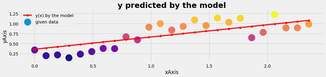
plot_gr02(xtest,ytest,xtest,y_pred_test,'xAxis','yAxis','y predicted by the model')
---- Linear Regression: resulting model parameters of training ----
Coefficient  :   [[0.30554815]]
Intercept     :  [0.35924642]

---- Test vs Training: check the score: ----
Training Score        :  0.468824081497367
Testing Score         :  0.6325095570532999
sTest-sTrain          :  0.16368547555593294
(sTest-sTrain)/sTrain :  0.34914050283667486
Logistic regression with 1 feature
Don’t get confused by its name! It is a classification not a regression algorithm. It is used to estimate discrete values ( Binary values like 0/1, yes/no, true/false ) based on given set of independent variables.
To the math: the log odds of the outcome is modeled as a linear combination of the predictor variables.
Above, p is the probability of the presence of the characteristic of interest. It chooses the parameters that maximize the likelihood of observing the sample values.
Generate data set
Again we use two data sets - training data - test data
NT = 26
xtrain,ytrain = generate_data_1D(NT,case=3)
xtest,ytest = generate_data_1D(NT,case=3)
# plot_gr01(xtrain,ytrain,'xAxis','yAxis','training data')
# plot_gr01(xtest,ytest,'xAxis','yAxis','test data')
Training
#--- train the model with the training data set
logist.fit(xtrain, ytrain.ravel());
Testing
#--- use the test data set and check the score with the model
score_training = logist.score(xtrain, ytrain)
score_testing = logist.score(xtest, ytest)
#--- display the model parameters
print('\n\n')
print('---- Logistic Regression: resulting model parameters of training ----')
print('Coefficient : ', logist.coef_)
print('Intercept : ', logist.intercept_)
print()
print('---- Test vs Training: check the score: ----')
print('Training Score : ', score_training)
print('Testing Score : ', score_testing)
print('sTest-sTrain : ', score_testing-score_training)
print('(sTest-sTrain)/sTrain : ', (score_testing-score_training)/score_training)
print('\n\n')
#--- predict y by the model
xmodel = np.linspace(np.min(xtest),np.max(xtest),NT).reshape(-1,1)
y_pred_test = logist.predict(xtest)
y_pred_model = logist.predict(xmodel)
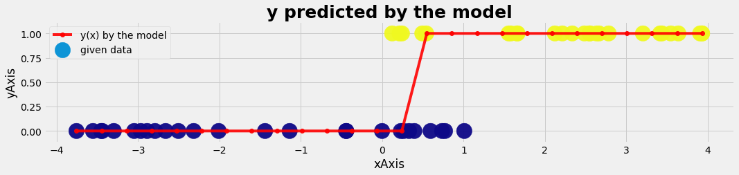
plot_gr02(xtest,ytest,xmodel,y_pred_model,'xAxis','yAxis','y predicted by the model')
---- Logistic Regression: resulting model parameters of training ----
Coefficient  :   [[1.78849999]]
Intercept     :  [-0.82190826]

---- Test vs Training: check the score: ----
Training Score        :  0.9230769230769231
Testing Score         :  0.8653846153846154
sTest-sTrain          :  -0.05769230769230771
(sTest-sTrain)/sTrain :  -0.06250000000000001
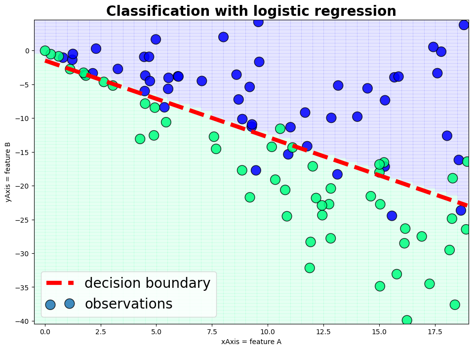
Logistic regression with 2 features
We just run through a logistic model with two features
#---- generate the data
x,y,v1 = generate_data_2D(NT=50, case=1);  X1 = np.vstack((x,y)).T   # 1 = training data
x,y,v2 = generate_data_2D(NT=50, case=1);  X2 = np.vstack((x,y)).T   # 2 = test data
#---- train the model
model = sl.linear_model.LogisticRegression(C=1e-1, solver='lbfgs')
model.fit(X1, v1);
#---- test the model
score_1 = model.score(X1, v1)
score_2 = model.score(X2, v2)
print('\n');print('Testing --------------')
print('score training :', score_1)
print('score test     :', score_2); print()
Testing --------------
score training : 0.82
score test     : 0.82
#--- evaluate the decision boundary
wght = model.coef_
icpt = model.intercept_
print('weights:    ', wght)
print('intercepts: ', icpt)
a1 = -wght[0,0]/wght[0,1]
b1 = icpt[0]/wght[0,1]
xm = np.r_[np.min(x),np.max(x)]
ym = a1*xm -b1

plot_gr03(x,y,v2,xm,ym,'xAxis = feature A','yAxis = feature B','Classification with logistic regression')
weights:     [[-0.33762703 -0.2979359 ]]
intercepts:  [-0.43771573]
Outlook
- we have used the historicaly earliest predictive models as an introduction
- there are more advanced models today
- to find a model with a high predictive power is a core issue
- since most models have some degrees of freedom (e.g. which degree of polynom do we use), we need a strategy to find the best model
- the training of the model depends on the data used too (resulting in overfitting and underfitting). So we need a strategy too for a systematic cross-validation and model fitting process.
- putting all this aspects together gives the learning curve of the algorithm as a guidance how to proceed.
--- Python code: Data generation
def generate_data_1D(NT, case=1):
    t0 = np.linspace(0,1,NT)
    if case == 1:
        x = 1.0 * t0;   a=0; b=0.5; y = a + b*x   # line
        rf = 0.1; y = y + rf*np.random.randn(len(y))
    if case == 2:
        x = t0 * 0.75 * np.pi;   y = np.sin(x)   # sinus
        rf = 0.15; y = y + rf*np.random.randn(len(y))
    if case==3:
        xp =  4* np.random.rand(NT); yp = np.ones_like(xp)
        xm = -5* np.random.rand(NT); ym = np.zeros_like(xm)
        overlap = 1.2
        x = np.hstack((xm+overlap,xp))
        y = np.hstack((ym,yp))
    x,y  = x.reshape(-1, 1), y.reshape(-1, 1)
    return x,y
def generate_data_2D(NT, case=1):
    t0 = np.linspace(0,1,NT)
    if case==1:
        L1=19.0; a1=  0; b1= -0.8;  rf1=0.5;
        L2=19.0; a2=  0; b2= -1.8;  rf2=0.5;

        x1 =  L1* np.random.rand(NT); r1 = a1 + b1*x1 ; y1 = r1 + rf1*x1* np.random.randn(NT); v1 = np.zeros_like(x1)
        x2 =  L2* np.random.rand(NT); r2 = a2 + b2*x2 ; y2 = r2 + rf2*x2* np.random.randn(NT); v2 = np.ones_like(x2)

        x = np.hstack((x1,x2)); y = np.hstack((y1,y2)); v = np.hstack((v1,v2))
    return x,y,v
--- Python code: Graphics
def plot_gr01(X,Y,xLabel,yLabel,grTitel):
    with plt.style.context('fivethirtyeight'):

         fig = plt.figure(figsize=(35,3)) ;

         ax1 = fig.add_subplot(121);
         a1size = np.ones_like(X)*500;

         ax1.scatter(X, Y, marker='o', s=a1size,  c=Y, edgecolors='w',cmap="plasma", alpha=0.95);
         #ax1.plot(X,Y,'b--',lw=1);

         plt.xlabel(xLabel);  plt.ylabel(yLabel);
         plt.title(grTitel, fontsize=25, fontweight='bold');
         #ax1.set_aspect('equal');
         plt.show()

def plot_gr02(X1,Y1,X2,Y2,xLabel,yLabel,grTitel):
    with plt.style.context('fivethirtyeight'):
         fig = plt.figure(figsize=(35,3)) ;
         ax1 = fig.add_subplot(121);
         a1size = np.ones_like(X1)*500;

         ax1.scatter(X1, Y1, marker='o', s=a1size,  c=Y1, #edgecolors='chartreuse', linewidths=2,
                     cmap="plasma", alpha=0.95, label='given data',zorder=1);
         ax1.plot(X2,Y2,'r-o',lw=4, alpha=0.9, label='y(x) by the model',zorder=2);

         plt.xlabel(xLabel);  plt.ylabel(yLabel);
         plt.legend()
         plt.title(grTitel, fontsize=25, fontweight='bold');
         #ax1.set_aspect('equal');
         plt.show()

def plot_gr03(X,Y,V,Xm,Ym,xLabel,yLabel,grTitel):
    with plt.style.context('fivethirtyeight'):
         fig = plt.figure(figsize=(25,8)) ;
         ax1 = fig.add_subplot(121);
         a1size = np.ones_like(X)*200;

         ax1.scatter(X, Y, marker='o', s=a1size,  c=V, edgecolors='k',cmap="winter",
                     alpha=0.85, zorder=2, label='observations');
         ax1.plot(Xm,Ym,'r--',lw=6, label='decision boundary');

         plt.xlabel(xLabel);  plt.ylabel(yLabel);
         plt.title(grTitel, fontsize=20, fontweight='bold');
         #ax1.set_aspect('equal');

         x_min, x_max = X.min()-0.5, X.max()+0.5
         y_min, y_max = Y.min()-0.5, Y.max()+0.5
         h = 0.5  # step size in the mesh
         xx, yy = np.meshgrid(np.arange(x_min, x_max, h), np.arange(y_min, y_max, h))
         Z = model.predict(np.c_[xx.ravel(), yy.ravel()])

         # Put the result into a color plot
         Z = Z.reshape(xx.shape)
         ax1.pcolormesh(xx, yy, Z, cmap='winter', alpha=0.1, zorder=1, label='model prediction')
         plt.legend(loc="lower left", scatterpoints=2, prop={'size': 20})
         plt.show()

# plot_gr03(x,y,v,xm,ym,'xAxis = feature A','yAxis = feature B','Classification with logistic regression')

def flowchart_1():
    fig = plt.figure(figsize=(20, 3), facecolor='w')
    ax = plt.axes((0, 0, 1, 1), frameon=False, xticks=[], yticks=[])   #

    dpx = 5.0; dpy = 1.0;
    polyF = 1.0
    polyG = polyF*np.array([[0.0, 1.0], [1.0, 0.0], [0.0, -1.0], [-1.0, 0.0] ])
    polyG[:,0] = polyG[:,0] + dpx;   polyG[:,1] = polyG[:,1] + dpy

    patches = [ Rectangle((1.0, 0.0), 1.0, 2.0, fc='c'),
                FancyArrow(2.5, 1.0, 1.0, 0, fc='m', width=0.5, head_width=0.95, head_length=0.2),
                Polygon(polyG, fc='gold'),
                FancyArrow(6.25, 1.0, 1.0, 0, fc='m', width=0.5, head_width=0.95, head_length=0.2),
                Rectangle((7.75, 0.0), 1.5, 2.0, fc='c', alpha=0.3),
              ]
    for p in patches:
        ax.add_patch(p)
    #ax.set_aspect('equal');
    plt.text(1.5, 1.1, "Features\nof the\nObjects", ha='center', va='center', fontsize=20)
    plt.text(5.0, 1.1, "Predictive\nModel", ha='center', va='center', fontsize=20)
    plt.text(8.5,1.1, "Names,\n Labels \n of the \n Objects\n\n (targets, classes)", ha='center', va='center', fontsize=20)
    plt.margins(0.1)

#flowchart_1()
Ressources
- http://openclassroom.stanford.edu/MainFolder/CoursePage.php?course=MachineLearning
- https://www.youtube.com/watch?v=mz3j59aJBZQ Andy Ng
- https://www.youtube.com/watch?v=gNhogKJ_q7U
- https://www.analyticsvidhya.com/blog/2017/09/common-machine-learning-algorithms/
- https://towardsdatascience.com/building-a-logistic-regression-in-python-301d27367c24
- http://christianherta.de/lehre/dataScience/machineLearning/logisticRegression.pdf
- https://www.tu-chemnitz.de/hsw/psychologie/professuren/method/homepages/ts/methodenlehre/LogistischeRegression.pdf
- https://www.statistik.uni-dortmund.de/fileadmin/user_upload/Lehrstuehle/Datenanalyse/Wissensentdeckung/Wissensentdeckung-Li-4_2x2.pdf