
- Di 07 März 2017
- MetaAnalysis
- Peter Schuhmacher
- #Statistics, #Bayes
Intro
The Bayesian rule
seems to be a rather abstract formula. But this impression can be corrected easely when considering a simple practical application. We call this approach mechanical because for this type of application there is no philosphical dispute between frequentist's and bayesian's mind set. We will just use in a mechanical/algorithmical manner the cells of a matrix. In this section we
- formulate a prototype of a probability problem (with red and green balls that have letters A and B printed on)
- summarize the problem in a basically 2x2 matrix (called contingency table)
- use the frequencies first
- replace them by probalities afterwards and recognize what conditional probablities are
- recognize that applying the Bayesian formula is nothing else than walking from one side of the matrix to the other side
A prototype of a probability problem
Given:
- 19 balls
- 14 balls are red, 5 balls are green
- among the 14 red balls, 4 have a A printed on, 10 have a B printed on
- among the 5 green balls, 1 has a A printed on, 4 have a B printed on
Typical questions: - we take 1 ball. - What is the probabilitiy that it is green ? - What is the probabilitiy that it is B under the precondition it's green ?
We will use Pandas to represent the problem and the solutions
import matplotlib.pyplot as plt
from IPython.core.pylabtools import figsize
import numpy as np
import pandas as pd
pd.set_option('precision', 3)
Contingency table with the frequencies
The core of the representation is a 2x2 matrix that summarizes the situation of the balls with the colors and the letters on. This matrix is expanded with the margins that contain the sums.
- sum L stands for the sum of the letters
- sum C stands for the sum of the colors
columns = np.array(['A', 'B'])
index   = np.array(['red', 'green'])
data    = np.array([[4,10],[1,4]])

df = pd.DataFrame(data=data, index=index, columns=columns)
df['sumC'] = df.sum(axis=1)  # append the sums of the rows
df.loc['sumL']= df.sum()     # append the sums of the columns
df
| A | B | sumC | |
|---|---|---|---|
| red | 4 | 10 | 14 |
| green | 1 | 4 | 5 |
| sumL | 5 | 14 | 19 |
Append the relative contributions of B and of green
We expand the matrix by a further column and a further row and use them to compute relative frequencies (see below).
def highlight_cells(x):
    df = x.copy()
    df.loc[:,:] = ''
    df.iloc[1,1] = 'background-color: #53ff1a'
    df.iloc[1,3] = 'background-color: lightgreen'
    df.iloc[3,1] = 'background-color: lightblue'
    return df

df[r'B/sumC']         = df.values[:,1]/df.values[:,2]
df.loc[r'green/sumL'] = df.values[1,:]/df.values[2,:]

t = df.style.apply(highlight_cells, axis=None)
t
| A | B | sumC | B/sumC | |
|---|---|---|---|---|
| red | 4 | 10 | 14 | 0.714 |
| green | 1 | 4 | 5 | 0.8 |
| sumL | 5 | 14 | 19 | 0.737 |
| green/sumL | 0.2 | 0.286 | 0.263 | 1.09 |
Let's focus on the row with the green balls
From all green balls (= 5) is the portion of those with a letter B (=4) 0.8
Note that this value already corresponds to the conditional probality \(P(B \mid green)\)
Let's focus on the column with the balls with letter B
From all balls with letter B (= 14) is the portion of those that are green (=4) 0.286
Note that also this value already corresponds to the conditional probality \(P(green \mid B)\)
Contingency table with the probabilities
We find the probabilities by dividing the frequencies by the sum of balls.
columns = np.array(['A', 'B'])
index   = np.array(['red', 'green'])
data    = np.array([[4,10],[1,4]])
data    = data/np.sum(data)

df = pd.DataFrame(data=data, index=index, columns=columns)
df['sumC'] = df.sum(axis=1)  # append the sums of the rows
df.loc['sumL']= df.sum()     # append the sums of the columns
df
| A | B | sumC | |
|---|---|---|---|
| red | 0.211 | 0.526 | 0.737 |
| green | 0.053 | 0.211 | 0.263 |
| sumL | 0.263 | 0.737 | 1.000 |
Append the relative contributions of B and of green
df[r'B/sumC']         = df.values[:,1]/df.values[:,2]
df.loc[r'green/sumL'] = df.values[1,:]/df.values[2,:]
t = df.style.apply(highlight_cells, axis=None)
t
| A | B | sumC | B/sumC | |
|---|---|---|---|---|
| red | 0.211 | 0.526 | 0.737 | 0.714 |
| green | 0.0526 | 0.211 | 0.263 | 0.8 |
| sumL | 0.263 | 0.737 | 1 | 0.737 |
| green/sumL | 0.2 | 0.286 | 0.263 | 1.09 |
Note the formula in the cells
columns = np.array(['-----------A----------', '---------B----------', '----------sumC--------',  '--------B/sumC--------'])
index   = np.array(['red', 'green', 'sumL',  'green/sumL'])
data    = np.array([['...','...','...','...'],
                    ['...', '$P(B \cap green)$', '$P(green)$', '$P(B \mid green)$'],
                    ['...','$P(B)$','...','...'],
                    ['...','$P(green \mid B)$','...','...'] ])
df = pd.DataFrame(data=data, index=index, columns=columns)
t = df.style.apply(highlight_cells, axis=None)
t
| -----------A---------- | ---------B---------- | ----------sumC-------- | --------B/sumC-------- | |
|---|---|---|---|---|
| red | ... | ... | ... | ... |
| green | ... | \(P(B \cap green)\) | \(P(green)\) | \(P(B \mid green)\) |
| sumL | ... | \(P(B)\) | ... | ... |
| green/sumL | ... | \(P(green \mid B)\) | ... | ... |
Conditional probability: Let's focus on the row with the green balls
The probability to get a ball with B out of all green balls is 0.8
Conditional probability: Let's focus on the column with the balls with letter B
The probability to get a green ball out of all balls with a B is 0.286
Bayes rule
Given \(P(green \mid B\)) find \(P(B \mid green)\) :
and given \(P(B \mid green)\) find \(P(green \mid B\)):
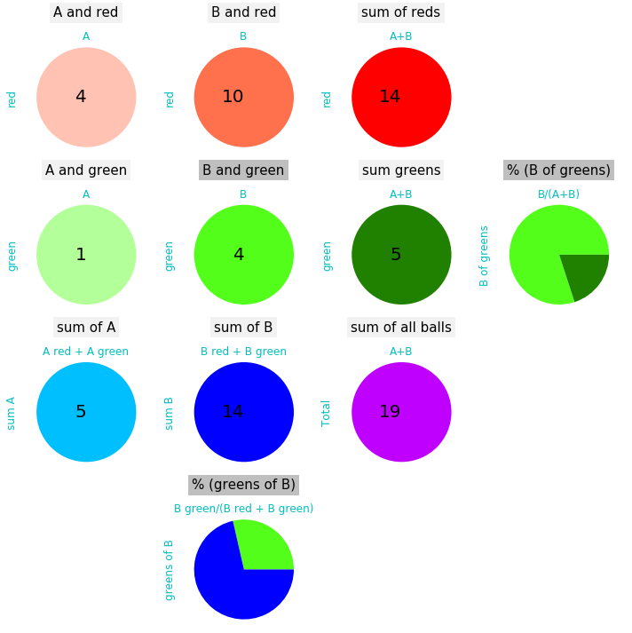
Applying the Bayes rule means that we walk from the element most right in the matrix to the element at the bottom of the matrix and vice versa:
show_frequencies()
def show_frequencies():
    px = 4; py = 4


    figsize(10, 10)
    fontSize1 = 15
    fontSize2 = 12
    fontSize3 = 20

    A1 = 4;     A2 = 10;       A3 = A1+A2
    B1 = 1;     B2 =  4;       B3 = B1+B2
    C1 = A1+B1; C2 = A2+B2;   C3 = A3+B3

    data = np.array([[A1, A2, A3],
                     [B1, B2, B3],
                     [C1, C2, C3] ])

    clr     = np.array([ ['#ffc2b3', '#ff704d', '#ff0000'],
                         ['#b3ff99', '#53ff1a', '#208000'],
                         ['#00bfff', '#0000ff', '#bf00ff']   ])


    title  = np.array([['A and red', 'B and red', 'sum of reds',
                       '$P(B|red) = \\frac {P(A\\cap red)}{P(red)}$'           ],
                       ['A and green', 'B and green', 'sum greens',   '% (B of greens)'     ],
                       ['sum of A', 'sum of B', 'sum of all balls',' '        ],
                       [' ', '% (greens of B)', '',  ' '     ],
                  ]  )

    xlabel = np.array([ ['A', 'B', 'A+B', 'B/(A+B)'],
                        ['A', 'B', 'A+B', 'B/(A+B)'],
                        ['A red + A green', 'B red + B green', 'A+B', 'B/(A+B)'],
                        ['A', 'B green/(B red + B green)', 'A+B', 'B/(A+B)']       ]  )

    ylabel = np.array([ ['red',   'red',   'red',  'B of reds'],
                        ['green', 'green', 'green','B of greens'],
                        ['sum A', 'sum B', 'Total', '' ],
                        ['green', 'greens of B', 'green', ' '],    ])


    f, ax = plt.subplots(px, py, sharex=True, sharey=True, edgecolor='none')  #, facecolor='lightgrey'

    for i in range(px-1):
        for j in range(py-1):

            patches, texts =ax[i,j].pie([data[i,j]], labels=[str(data[i,j])], #autopct='%1.1f%%',
                            shadow=False, startangle=90, labeldistance=0.0,
                            colors = [clr[i,j]])
            texts[0].set_fontsize(fontSize3)
            ax[i,j].set_title(title[i,j], position=(0.5,1.2), bbox=dict(facecolor='#f2f2f2', edgecolor='none'), fontsize= fontSize1)
            if i*j==1 :
                ax[i,j].set_title(title[i,j], position=(0.5,1.2), bbox=dict(facecolor='#bfbfbf', edgecolor='none'), fontsize=fontSize1)

            ax[i,j].set_xlabel(xlabel[i,j], fontsize=fontSize2, color='c')
            ax[i,j].xaxis.set_label_position('top')

            ax[i,j].set_ylabel(ylabel[i,j], fontsize=fontSize2, color='c')

            ax[i,j].axis('equal')

        j += 1
        if (i == 1):
            p = data[i,-2]/data[i,-1]; o = p/(1-p)
            patches, texts =ax[i,j].pie([o,1], #autopct='%1.1f%%',
                            shadow=False, startangle=0.0, labeldistance=0.0,
                            colors = [clr[i,1], clr[i,2] ] )
            texts[0].set_fontsize(fontSize3)
            ax[i,j].set_title(title[i,j], position=(0.5,1.2), bbox=dict(facecolor='#bfbfbf', edgecolor='none'), fontsize=fontSize1)
            ax[i,j].set_xlabel(xlabel[i,j], color='c', fontsize=fontSize2)
            ax[i,j].xaxis.set_label_position('top')
            ax[i,j].set_ylabel(ylabel[i,j], fontsize=fontSize2, color='c')
            ax[i,j].axis('equal')
        else:
            ax[i,j].plot(0,0)
            ax[i,j].set_frame_on(False)

    i = px-1;
    for j in range(py):
        if j==1:
            p = data[1,1]/data[2,1]; o = p/(1-p)
            patches, texts =ax[i,j].pie([o,1], #autopct='%1.1f%%',
                        shadow=False, startangle=0.0, labeldistance=0.0,
                        colors = [clr[1,1], clr[2,1] ])
            texts[0].set_fontsize(fontSize3)
            ax[i,j].set_title(title[i,j], position=(0.5,1.2), bbox=dict(facecolor='#bfbfbf', edgecolor='none'), fontsize=fontSize1)

            ax[i,j].set_xlabel(xlabel[i,j], color='c', fontsize=fontSize2)
            ax[i,j].xaxis.set_label_position('top')
            ax[i,j].set_ylabel(ylabel[i,j], fontsize=fontSize2, color='c')
            ax[i,j].axis('equal')
            ax[i,j].set_facecolor('y')
        else:
            ax[i,j].plot(0,0)
            ax[i,j].set_frame_on(False)

    plt.tight_layout()
    plt.show()
from IPython.display import HTML

# HTML('''<script> $('div .input').hide()''') #lässt die input-zellen verschwinden

HTML('''<script>
code_show=true;
function code_toggle() {
 if (code_show){
 $('div.input').hide();
 } else {
 $('div.input').show();
 }
 code_show = !code_show
}
$( document ).ready(code_toggle);
</script>
<form action="javascript:code_toggle()"><input type="submit" value="Click here to toggle on/off the raw code."></form>''')