
- Mi 08 März 2017
- MetaAnalysis
- Peter Schuhmacher
- #Statistics, #Python
%matplotlib inline
from IPython.core.pylabtools import figsize
from matplotlib import pyplot as plt
import numpy as np
import scipy.stats as st
import seaborn
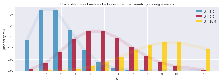
Poisson distribution
$$
P_{\lambda }(k)={\frac {\lambda ^{k}}{k!}}\,{\mathrm {e}}^{{-\lambda }}
$$
figsize(12.5, 4)

a  = np.linspace(0, 12, 12, dtype=int)
poi = st.poisson

lambda_ = [2.0, 5.0, 10.0]
colours = ["#348ABD", "#A60628","#ffcc00", "#66ff33"]
dx = 0.3
ds = 1*dx

for k, N in enumerate(lambda_):

    plt.bar(a+k*ds, poi.pmf(a, lambda_[k]), label="$\lambda = %.1f$" % lambda_[k],
            width = dx,
            color=colours[k], alpha=0.80,
            edgecolor=colours[k], lw="0")
    plt.plot(a+k*ds, poi.pmf(a, lambda_[k]), color=colours[k], #label="$\lambda = %.1f$" % lambda_[k],
            lw=10, alpha=0.1)
plt.xticks(a + 0.4, a)
plt.legend()
plt.ylabel("probability of $k$")
plt.xlabel("$k$")
plt.title("Probability mass function of a Poisson random variable; differing \
$\lambda$ values");
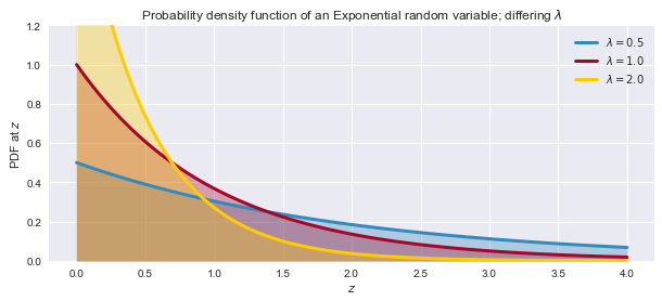
Exponential Distribution
$$
f_{{\lambda }}(x)={\begin{cases}\displaystyle \lambda {{\rm {e}}}^{{-\lambda x}}&x\geq 0\\0&x<0\end{cases}}
$$
figsize(10, 4)
colours = ["#348ABD", "#A60628","#ffcc00", "#66ff33"]
a = np.linspace(0, 4, 100)
expo = st.expon
lambda_ = [0.5, 1, 2]

for k, c in zip(lambda_, colours):
    plt.plot        (a, expo.pdf(a, scale=1./k), color=c, lw=3,     label="$\lambda = %.1f$" % k)
    plt.fill_between(a, expo.pdf(a, scale=1./k), color=c, alpha=.33 )

plt.legend()
plt.ylabel("PDF at $z$")
plt.xlabel("$z$")
plt.ylim(0, 1.2)
plt.title("Probability density function of an Exponential random variable;\
 differing $\lambda$");
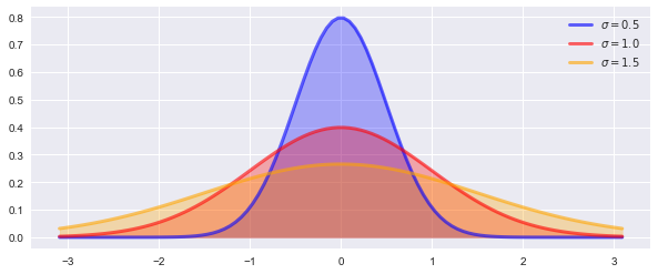
Normal Distribution
$$
f(x)={\frac {1}{\sigma {\sqrt {2\pi }}}}e^{-{\frac {1}{2}}\left({\frac {x-\mu }{\sigma }}\right)^{2}}
$$
μ = 0.0      #mean
σ = 1.0      #standard deviation
α = 0.05     #significance level

distrib = st.norm(μ, σ)
φ = distrib.ppf([0.5*α , 1.0-0.5*α])
print(φ )

colours = ['blue', 'red', 'orange']
μ = 0.0                                 #mean
σ_array = [0.5, 1.0, 1.5]               #standard deviation
x = np.linspace(st.norm.ppf(0.001), st.norm.ppf(0.999), 100)

figsize(10, 4)
fig, ax = plt.subplots(1, 1)
for σ, c in zip(σ_array, colours):
    ax.plot(x, st.norm.pdf(x,μ, σ),color=c, lw=3, alpha=0.6, label="$σ = %.1f$" % σ)
    ax.fill_between(x, st.norm.pdf(x, μ, σ),color=c, alpha=0.3)

ax.legend(loc='best', frameon=False)
plt.show()
[-1.95996398 1.95996398]
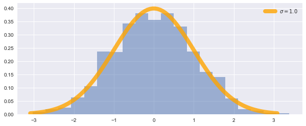
Randomly generated normal distribution
import seaborn as sns

μ = 0.0      #mean
σ = 1.0      #standard deviation
nBins = 20   # number of classes in histogram

# get random samples
nSamples = 1000
normD =  st.norm(μ, σ)               # generate dats
trials = normD.rvs(nSamples)        # take a random sample out of the data

# draw pdf
x = np.linspace(st.norm.ppf(0.001), st.norm.ppf(0.999), 100)
figsize(10, 4)
fig, ax = plt.subplots(1, 1)
ax.plot(x, st.norm.pdf(x,μ, σ),color='orange', lw=8, alpha=0.8, label="$σ = %.1f$" % σ)
ax.legend(loc='best', frameon=False)

# draw histogram
plt.hist(trials,nBins, normed=True,alpha=0.5);
plt.show()
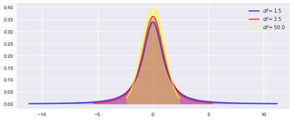
t-Distribution
$$
{\displaystyle f_{n}(x)={\frac {\Gamma \left({\frac {n+1}{2}}\right)}{{\sqrt {n\pi }}~\Gamma \left({\frac {n}{2}}\right)}}\left(1+{\frac {x^{2}}{n}}\right)^{-{\frac {n+1}{2}}}}
$$
$$
with \;\;\; \Gamma(x)=\int\limits_{0}^{+\infty}t^{x-1}e^{-t}\operatorname{d}t
$$
#colours = ["#348ABD", "#A60628","#ffcc00", "#66ff33"]
colours = ['blue', 'red', 'yellow']
DoF = [1.5, 2.5, 50.0]    # degree of freedom

figsize(10, 4)
fig, ax = plt.subplots(1, 1)
for df, c in zip(DoF, colours):
    x = np.linspace(st.t.ppf(0.01, df), st.t.ppf(0.99, df), 100)
    ax.plot(x, st.t.pdf(x, df),color=c, lw=3, alpha=0.6, label=("$df = %.1f$" % df))
    ax.fill_between(x, st.t.pdf(x, df),color=c, alpha=0.3)

ax.legend(loc='best', frameon=False)
plt.show()
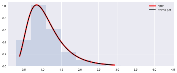
F-Distribution \({\displaystyle F(m,n)}\)
with m degree of freedoms in the numerator and n degrees of freedom in the denominator
$$
{\displaystyle F(x|m,n)={\begin{cases}m^{\frac {m}{2}}n^{\frac {n}{2}}\cdot {\frac {\Gamma ({\frac {m}{2}}+{\frac {n}{2}})}{\Gamma ({\frac {m}{2}})\Gamma ({\frac {n}{2}})}}\cdot {\frac {x^{{\frac {m}{2}}-1}}{(mx+n)^{\frac {m+n}{2}}}}&{\text{if}}\;x\geq 0\\0&{\text{else}}\\\end{cases}}}
$$
$$
with \;\;\; \Gamma(x)=\int\limits_{0}^{+\infty}t^{x-1}e^{-t}\operatorname{d}t
$$
figsize(10, 4)
fig, ax = plt.subplots(1, 1)

# set degree of freedom in numerator, denominator
dfn, dfd = 29, 18

# Display the probability density function (pdf):
x = np.linspace(st.f.ppf(0.01, dfn, dfd),
                st.f.ppf(0.99, dfn, dfd), 300)
ax.plot(x, st.f.pdf(x, dfn, dfd),
          'r-', lw=5, alpha=0.6, label='f pdf')

# Freeze the distribution and display the frozen pdf:
rv = st.f(dfn, dfd)   # random variable
ax.plot(x, rv.pdf(x), 'k-', lw=2, label='frozen pdf')

# generate f-distributed random numbers...
randF = st.f.rvs(dfn, dfd, size=1000)

# ...and draw histogram
ax.hist(randF, normed=True, histtype='stepfilled', alpha=0.2)

ax.legend(loc='best', frameon=False)
plt.show()
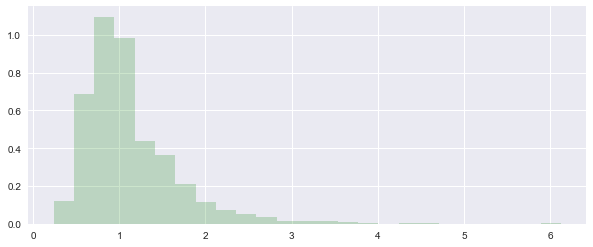
Random F-Distribution \({\displaystyle F(m,n)}\) with numpy
figsize(10, 4)
dfnum = 29. # between group degrees of freedom
dfden = 18. # within groups degrees of freedom
nBins = 25
s = np.random.f(dfnum, dfden, 1000)
plt.hist(s, nBins,normed=True, histtype='stepfilled', facecolor='green', alpha=0.2);
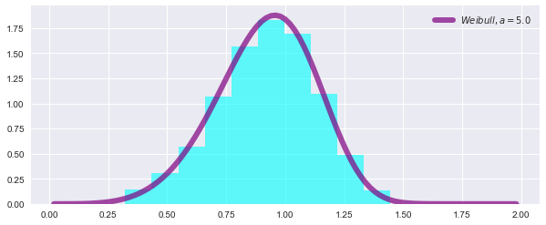
Random Weibull-Distribution with numpy
$$
f(x)=\lambda \cdot k\cdot (\lambda \cdot x)^{{k-1}}{\mathrm {e}}^{{-(\lambda \cdot x)^{k}}}
$$
# get random sample and plot histogram
figsize(10, 4)
a = 5. # shape
s = np.random.weibull(a, 1000)
plt.hist(s, normed=True, histtype='stepfilled', facecolor='cyan', alpha=0.6);

# plot pdf
def weib(x,n,a):
    return (a / n) * (x / n)**(a - 1) * np.exp(-(x / n)**a)

x = np.arange(1,100.)/50.
weibullD = weib(x, 1., a)
plt.plot(x, weibullD, lw=6, alpha=0.7, color='purple',label=("$Weibull, a = %.1f$" % a))
plt.legend(loc='best', frameon=False)
plt.show()
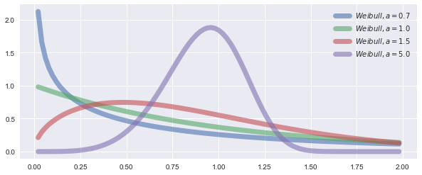
Weibull-Distribution with different parameters
figsize(15, 9)
figsize(10, 4)
A = [0.7, 1.0, 1.5, 5.0]
for  a in A:
    weibullD = weib(x, 1., a)
    plt.plot(x, weibullD, lw=7, alpha=0.6,label=("$Weibull, a = %.1f$" % a))

plt.legend(loc='best', frameon=False)
plt.show()
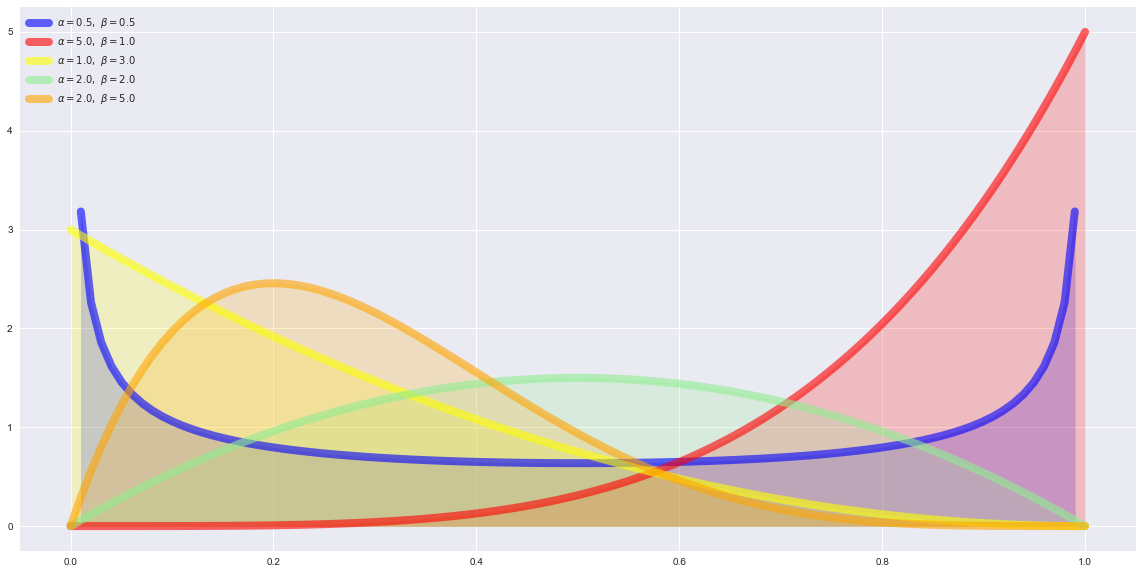
Beta-Distribution
$$
{\displaystyle f(x)={\frac {1}{B(p,q)}}x^{p-1}(1-x)^{q-1}={\frac {1}{B(p,q)}}x^{ α }(1-x)^{β}.}
$$
$$
with \;\;\; {\displaystyle B(p,q)={\frac {\Gamma (p)\Gamma (q)}{\Gamma (p+q)}}}
$$
$$
with \;\;\; \Gamma(x)=\int\limits_{0}^{+\infty}t^{x-1}e^{-t}\operatorname{d}t
$$
P = (0.5, 5, 1, 2, 2) # α
Q = (0.5, 1, 3, 2, 5) # β
colours = ['blue', 'red', 'yellow', 'lightgreen', 'orange']

figsize(20,10)
fig, ax = plt.subplots(1, 1)
for p, q, c in zip(P, Q, colours):
    x = np.linspace(st.beta.ppf(0.00, p, q), st.beta.ppf(1, p, q), 100)
    ax.plot(x, st.beta.pdf(x, p, q), color=c, lw=8, alpha=0.6,  label=r'$\alpha=%.1f,\ \beta=%.1f$' % (p, q))
    ax.fill_between(x, st.beta.pdf(x, p, q),color=c, alpha=0.2)

plt.legend(loc='best', frameon=False)
PL= [2.0, 5.0, 10.0]
Binomial distribution
$$
B\; (k \mid n,p)=\binom nk\cdot p^k\cdot (1-p)^{n-k}
$$
B is the probability of k succesful events given n trials and the probability p of a single event.