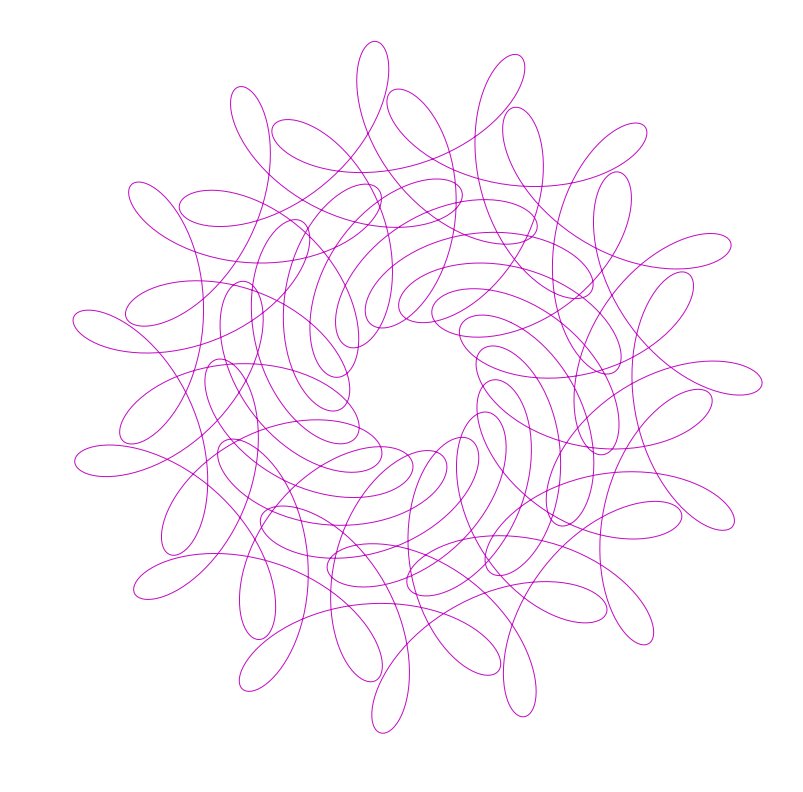
I have found some fascinating "mystery curves" in this blog. The basic structure is a circle, but the radius is changing artfully too. The result is an ornamental curve in the 2-dimensional plane.

The Maths

The mathematical expression is

$$ f(t) = e^{it}\left[ 1 - \frac{1}{2}e^{ikt} + \frac{i}{3}e^{-ikt} \right] $$

The two components of the 2-dimensional plane, $(x,y)$, are summarized by the complex number $i$

$$ f = f(x,iy) $$

The discrete evaluation of the curve needs a resolution that is fine enough so that the curve is well-represented.

Steps towards the Arts

Some artistic effetcs can be attained by the following manipulations:

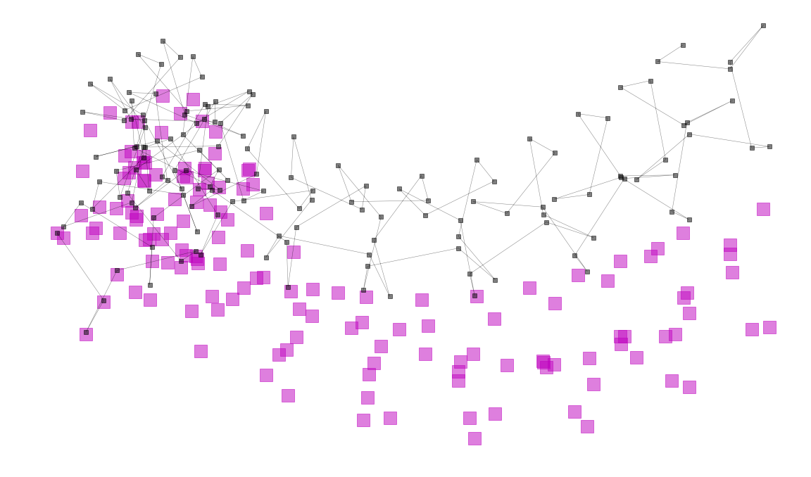
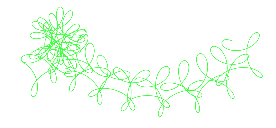
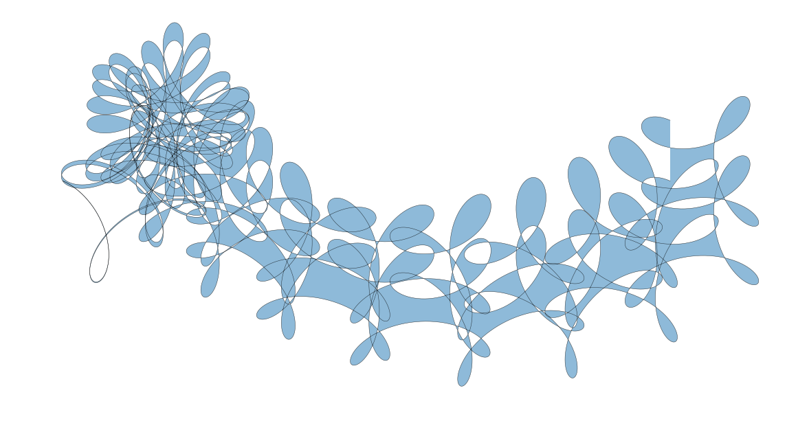
we expand the equation by adding some linear translations. So $f$ becomes $\tilde{f} = f(x,iy) + (a_1 \cdot x \, , \, a_2 \cdot y)$. The basic circular pattern is broken now, but we still have a non-random coherent structure.
we play around with the resolution. If the resolution is lowered, we get the impression of "a somehow controlled randomness" .
we use different styles to display (lines, points, collors, transparency)
we can plot two curves in the same canvas with slightly different parameters. This generates self-similarity

Below the code and some examples:

import sys
import matplotlib.pyplot as plt
import numpy as np

def f(t, k):
    # https://scipython.com/blog/the-mystery-curve/
    def P(z):   return 1 - z / 2 - 1 / z**3 / 3j
    return np.exp(1j*t) * P(np.exp(k*1j*t))

def generate_curve(res,k,case):
    t = np.linspace(0, 2*np.pi, res*k +1);
    u = f(t, k)
    # ---- graphics ----
    fig, ax = plt.subplots(figsize=(20,14), facecolor='w')
    if case=='A':
        #ax.scatter(np.real(u)+t, np.imag(u), s=300, marker='s', color='m', alpha=0.5)
        ax.plot(np.real(u), np.imag(u), lw=1, ls='-', color='m', alpha=0.95)
    if case=='B':
        vx1, vy1 = np.real(u)+t, np.imag(u)+0.1*t
        ax.plot(vx1, vy1 , lw=2.5, ls='-', color='lime', alpha=0.75)
    if case=='C':
        vx1, vy1 = np.real(u)+t, np.imag(u)+0.1*t
        vx2, vy2 = np.real(u)+t, np.imag(u)+0.0*t
        ax.plot(vx1, vy1 , lw=0.5, ls='-', color='k', alpha=0.75)
        ax.plot(vx2, vy2,  lw=0.5, ls='-', color='k', alpha=0.75)
        ax.fill_between(vx1,vy1,vy2, alpha=0.5)
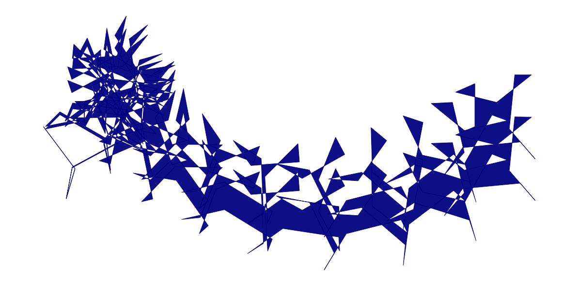
    if case=='D':
        vx1, vy1 = np.real(u)+t, np.imag(u)+0.1*t
        vx2, vy2 = np.real(u)+t, np.imag(u)+0.0*t
        ax.fill_between(vx1,vy1,vy2, color='navy', alpha=0.95)
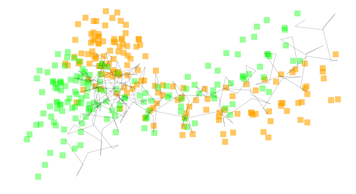
    if case=='E':
        vx1, vy1 = np.real(u)+t, np.imag(u)
        vx2, vy2 = np.real(u)+t-1.0, np.imag(u)+0.5*t-2.0

        ax.scatter(vx1, vy1, s=300, marker='s', color='orange', alpha=0.6)
        ax.scatter(vx2, vy2, s=300, marker='s', color='lime', alpha=0.4)
        ax.plot(   vx1, vy2, lw=0.5, ls='-', color='k', alpha=0.75)
    if case=='F':
        vx1, vy1 = np.real(u)+t, np.imag(u)
        vx2, vy2 = np.real(u)+t, np.imag(u)+0.3*t
        ax.scatter(vx1, vy1 , s=300, marker='s', color='m', alpha=0.5)
        ax.plot(   vx2, vy2 , lw=0.5, ls='-', marker='s', color='k', alpha=0.5)

    ax.set_aspect('equal')
    plt.axis('off')
    plt.savefig('mystery_curve_{}_{}_{}.png'.format(case,res,k))
    plt.show()

res, k = 201,15
generate_curve(res,k,'A')

png

res, k = 202,15
generate_curve(res,k,'B')

png

res, k = 203,15
generate_curve(res,k,'C')

png

res, k = 11,15
generate_curve(res,k,'D')

png

res, k = 10,15
generate_curve(res,k,'E')

png

res, k = 10,15
generate_curve(res,k,'F')

png

HealthyNumerics

The decorative side of mathematical functions

The Maths

Steps towards the Arts