NumericalStats: WHY to switch from a decision tree to a Markov model

So 25 März 2018
MetaAnalysis
Peter Schuhmacher
#numerical, #statistics, #python, #markov model

import numpy as np
import pandas as pd
from scipy import stats
from matplotlib import pyplot as plt
import matplotlib.colors as mclr

Why a change could be indicated

The decision tree is a simple form of decision model. But there are also limitions of the decision tree evident:

a formal aspect is that the tree format becomes rapidly unwiedly when a combination of several options have to be mapped
with regard to content the elapse of time is not explicit in decision trees. Many chronic diseases such as diabetes, ischaemic heart disease or some forms of cancer have a recuring-remitting pattern over a period of many years. If a longer time horizon has to be adopted, several features may become necessary to be modelled:
- continuing risk of recurrence
- competing risk of death as the cohort ages
- other clinical developments

The Markov model is an approach to handel added modelling options. The key structure of a markov model is:

it is structured around disease states
it is driven by a set of possible transitions between the disease states
it can be run over a series of time periods which gives an insight over the temporal evolution of the disease states
costs may be included in parallel
the modelled transistions probabilities may change over time too, so that changing conditions may be included

We give in the follwing a basic example of a Markov model that illustrates the temporal evolution of a communicable disease in a population.

$$ \begin{equation} \begin{array}{rcl} \textrm{Markov matrix} \; \mathbf{M} &=& \left[\begin{matrix}0.721 & 0.202 & 0.067 & 0.010 \\ 0.000 & 0.581 & 0.407 & 0.012 \\ 0.000 & 0.000 & 0.750 & 0.250 \\ 0.000 & 0.000 & 0.000 & 1.000 \end{matrix}\right] \\ \textrm{Start vector} \;\; \mathbf{p}_0 &=& \left[\begin{matrix}1 \\ 0 \\0 \\0\end{matrix}\right]\\ Repeat:\\ \textrm{Time step} \;\; \mathbf{p}_1 &=& \mathbf{M}^T \cdot \mathbf{p}_0 \\ \textrm{Iteration} \;\; \mathbf{p}_0 &:=& \mathbf{p}_1 \end{array} \end{equation} $$

d1

svg

Set up the Markov system

M_states = np.array(['A (healthy)', 'B (infected)', 'C (ill)', 'D (dead)'])
MM = np.array([[0.721,  0.202,  0.067,  0.010],
               [0.000,  0.581,  0.407,  0.012],
               [0.000,  0.000,  0.750,  0.250],  
               [0.000,  0.000,  0.000,  1.000] ])
dmm = pd.DataFrame(MM, columns=M_states, index=M_states); dmm

	A (healthy)	B (infected)	C (ill)	D (dead)
A (healthy)	0.721	0.202	0.067	0.010
B (infected)	0.000	0.581	0.407	0.012
C (ill)	0.000	0.000	0.750	0.250
D (dead)	0.000	0.000	0.000	1.000

Run the Markov simulation

We run the simulation with a population of 1000 members. Note that simulation part has 7 lines of code only:

nRuns = 21
m_result = np.zeros((nRuns,len(M_states)))
v0 = np.array([1, 0, 0, 0])*1000
for ir in range(nRuns):
    m_result[ir,:] = v0
    v0 = np.dot(MM.T,v0) 
dmr = pd.DataFrame(np.rint(m_result).astype(int), columns=M_states)

Plot the result

plot_gr02(dmr,'time','# of people','Markov simulation of a communicable disease'); dmr

png

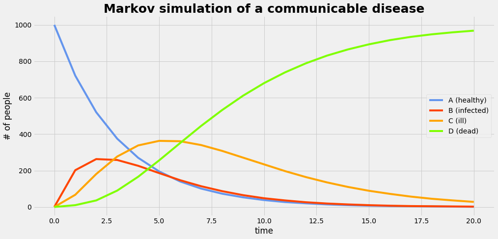
	A (healthy)	B (infected)	C (ill)	D (dead)
0	1000	0	0	0
1	721	202	67	10
2	520	263	181	36
3	375	258	277	90
4	270	226	338	166
5	195	186	363	256
6	140	147	361	351
7	101	114	340	445
8	73	87	308	532
9	53	65	271	611
10	38	48	234	680
11	27	36	197	739
12	20	26	164	789
13	14	19	135	831
14	10	14	110	865
15	7	10	89	893
16	5	7	72	916
17	4	5	57	934
18	3	4	45	948
19	2	3	36	959
20	1	2	28	968

import graphviz as gv
def plotMarkovModel():
    d1 = gv.Digraph(format='png',engine='dot')
    c = ['cornflowerblue','orangered','orange','chartreuse']
    d1.node('A','A (healthy)', style='filled', color=c[0])
    d1.node('B','B (infected)',style='filled', color=c[1])
    d1.node('C','C (ill)',     style='filled', color=c[2])
    d1.node('D','D (dead)',    style='filled', color=c[3])
    d1.edge('A','A',label='0.721'); d1.edge('A','B',label='0.202'); d1.edge('A','C',label='0.067'); d1.edge('A','D',label='0.010')
    d1.edge('B','B',label='0.581');                                 d1.edge('B','C',label='0.407'); d1.edge('B','D',label='0.012')
    d1.edge('C','C',label='0.750');                                                                 d1.edge('C','D',label='0.250')
    d1.edge('D','D',label='1.000');
    return d1
d1 = plotMarkovModel()
d1.render('img/mamo1', view=True)

def plot_gr02(DF,xLabel,yLabel,grTitel):
    with plt.style.context('fivethirtyeight'): 
         fig = plt.figure(figsize=(15,7)) ;
         ax1 = fig.add_subplot(111);
         #DF.plot(ax = plt.gca())
         colors = ['cornflowerblue','orangered','orange','chartreuse']
         DF.plot(ax = ax1, style='-', color=colors)
         plt.xlabel(xLabel);  plt.ylabel(yLabel);
         plt.title(grTitel, fontsize=25, fontweight='bold');
         plt.show()