
- Di 17 Dezember 2019
- MachineLearning
- Peter Schuhmacher
- #numerical, #statistics, #machine learning, #python
We present a solution method, the Stochastic Gradient Descent (SGD). Our approach is based on this repos:
- https://github.com/elizavetasemenova/amld-2019
- https://github.com/gregunz/AMLD2019/blob/master/workshops/02%20-%20Pneumonia%20Detection%20using%20CNN%20and%20pre-trained%20networks/1_gradient_descent/p2_gradient_example.ipynb
which we have slightly modified.
This is an iterative approach, in which the desiered solution is successively approached with every iteration. The gradient of the loss or error function gives the direction to control the development of the solution of the algorithm.
As an example we choose a linear 1-dimensional function to approach the data, which corresponds to a linear interpolation. The aim is to evaluate the model parameters \(\theta_0\) and \(\theta_1\) as slope and intercept.
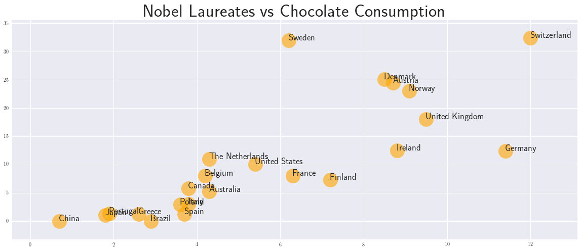
The data we use is from a paper published in New England Journal of Medicine. The author Franz Messerli reports a highly significant correlation between a nation's per capita chocolate consumption and the rate at which its citizens win Nobel Prizes. He reported "a close, significant linear correlation (r=0.791, p<0.0001) between chocolate consumption per capita and the number of Nobel laureates per 10 million persons in a total of 23 countries."
import numpy as np
import pandas as pd
from scipy import stats
import matplotlib.pyplot as plt
import random
from matplotlib import rc
rc('text', usetex=True)
print('\n\n\n')
data_df = pd.read_csv('data.csv')
nd = data_df.shape[0]
with plt.style.context('seaborn'):      # 'fivethirtyeight'
    fig = plt.figure(figsize=(20,8)) ;
    for i in range(nd):
        x = data_df.loc[i,data_df.columns[1]]
        y = data_df.loc[i,data_df.columns[2]]
        tx= data_df.loc[i,data_df.columns[0]]
        plt.plot(x, y, marker='o',ms=29, c='orange',alpha = 0.6)
        plt.text(x,y, tx, fontsize=18)
    plt.title('Nobel Laureates vs Chocolate Consumption', fontweight='bold',fontsize=35)
    plt.margins(0.1)
    plt.show()
1. Target function with parameters
We define the linear function f(x) that will approximate our dataset. It depends on two unknown parameters that we want to find out: \(\theta_0\) and \(\theta_1\):
\(f(x)=\theta_0 + \theta_1x\)
In matrix notation we can write
\(\mathbf{f}(\mathbf{x}) = \theta_0 + \theta_1 \mathbf{x}\)
2. Loss function
We define the loss or error function as the squared distance between the observed data \(y\) and its approximated value \(f(x)\)
\(L(\theta)=\sum_{i^{(i)}\in data} (f(x^{(i)}) - y^{(i)})^2\)
In matrix notation we can express this as a scalar product of the difference \(\mathbf{\delta} = \mathbf{f}(\mathbf{x})-\mathbf{y}\) which can be used for an implementation in vectorized form
\(L(\theta)=<\mathbf{\delta},\mathbf{\delta}>\) , scalar product
3. Derivatives of the loss function
They will be used for the descendent gradient algorithm
\(\frac{\partial L}{\partial \theta_0} = 2\sum_i (f(x^{(i)}) - y^{(i)})\)
and
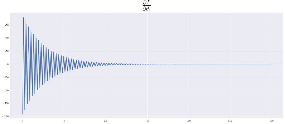
\(\frac{\partial L}{\partial \theta_1} = 2\sum_i (f(x^{(i)}) - y^{(i)})x_{1}^{(i)}\)
We implement these as
\(L_{\theta_0} = 2\cdot sum(\mathbf{\delta})\)
\(L_{\theta_1} = 2\cdot <\mathbf{\delta} , \mathbf{x} >\) , scalar product
4. Algorithm
It's a marching algorithm. Starting with some intitial values for \(\theta_0\) and \(\theta_1\) these are updated recursively:
\(\theta_0^{n+1} = \theta_0^n + \epsilon \frac{\partial L}{\partial \theta_0}\)
\(\theta_1^{n+1} = \theta_1^n + \epsilon \frac{\partial L}{\partial \theta_1}\)
We apply the standard approach where all data are used at each time step. There are variations in using only a subset of the data that are randomly picked out at each time step.
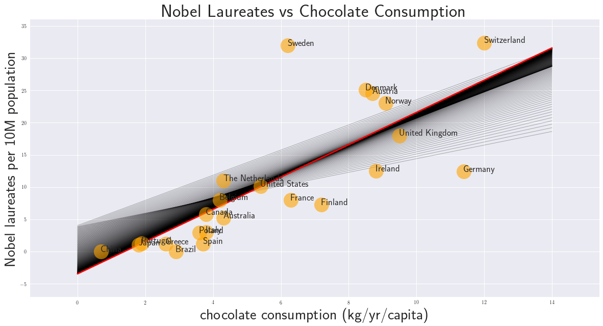
5. Solution
The rate of convergance depends on the choice of \(\epsilon\). With a low value the convergence is slow and many iterations are needed. With a large value to soltuion might oscillate or even diverge. This phenomena is well known in computational fluid dynamics where the Courant–Friedrichs–Lewy (CFL) condition is a necessary condition for convergence.
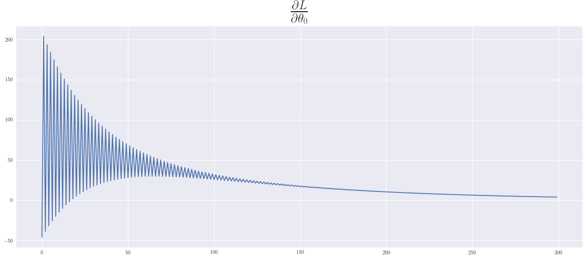
In playing around with this example we can see, that the convergence for the intercept is slower than for the slope. We have chosen \(\epsilon\) as large as possible, so that an oscillatory behaviour can be seen, which in this case is still benefical and supports a faster convergence.
A Runge-Kutta schema might improve the convergence properties.
def f(x,θ):
    return θ[0] + θ[1]*x

def f_loss(xs, ys,θ):
    delta = f(xs,θ) - ys
    return np.dot(delta,delta)

def f_dθ0(xs, ys,θ):
    return 2 * np.sum(f(xs,θ) - ys)

def f_dθ1(xs, ys,θ):
    delta = f(xs,θ) - ys
    return 2*np.dot(delta,xs)
data_df = pd.read_csv('data.csv')    # get the data
xs = np.array(data_df.values[:, 1],dtype=float)
ys = np.array(data_df.values[:, 2],dtype=float)

ε = 0.001                            # choose the time step
θ = np.array([4.0, 1.0])             # initialize the parameters theta
dLs, dT0, dT1 = [], [], []
loss_old = 1.0
print('\n\n\n')

with plt.style.context('seaborn'):
    fig = plt.figure(figsize=(20,10))
    x0, x1 = 0, 14                    # 2 x-points of the straight line in the graphics

    for i in range(300): #------------- run the algorithm -----------
        dθ0 = f_dθ0(xs, ys, θ)        # compute the gradients of theta
        dθ1 = f_dθ1(xs, ys, θ)
        dT0.append(dθ0)
        dT1.append(dθ1)

        θ[0] -= ε * dθ0               # update theta
        θ[1] -= ε * dθ1

        loss_new = f_loss(xs, ys, θ)  # check the development of the error
        dL = (loss_new-loss_old)/loss_old
        dLs.append(np.sqrt(dL*dL))
        loss_old = loss_new

        # ----- Graphics -------------------------------------------------
        plt.plot([x0, x1], [f(x0,θ), f(x1,θ)], 'k-', lw=1, alpha=0.3)
    plt.plot([x0, x1], [f(x0,θ), f(x1,θ)], 'r-', lw=3, alpha=0.93)

    for i in range(nd):
        x = data_df.loc[i,data_df.columns[1]]
        y = data_df.loc[i,data_df.columns[2]]
        tx= data_df.loc[i,data_df.columns[0]]
        plt.plot(x, y, marker='o',ms=29, c='orange',alpha = 0.6)
        plt.text(x,y, tx, fontsize=18)
    plt.xlabel(data_df.columns[1],size=30);
    plt.ylabel(data_df.columns[2],size=30)
    plt.title('Nobel Laureates vs Chocolate Consumption', fontweight='bold',fontsize=35)
    plt.margins(0.1)
    plt.show()

#---- compare with linear regression ---------
theta1, theta0,_,_,_  = stats.linregress(xs,ys)
fp = np.polyfit(xs,ys,1)
print('\n\n\n')
print("The parameters θ                        =",θ[1],θ[0])
print("The parameters with linear regression:  =",theta1, theta0)
print("The parameters with np.polyfit:         =",fp[0],fp[1])
print('\n\n\n')
The parameters θ                        = 2.501848008865261 -3.448185705127312
The parameters with linear regression:  = 2.548736915671354 -3.792170212097653
The parameters with np.polyfit:         = 2.548736915671355 -3.792170212097653
with plt.style.context('seaborn'):
fig = plt.figure(figsize=(20,8)) ;
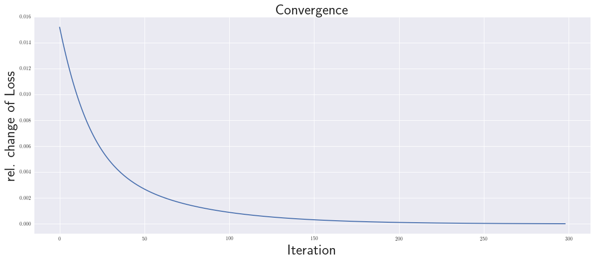
plt.plot(dLs[1:], lw=2)
plt.xlabel('Iteration',size=30); plt.ylabel('rel. change of Loss',size=30)
plt.title('Convergence',fontweight='bold', fontsize=30);
plt.show()
fig = plt.figure(figsize=(20,8)) ;
plt.plot(dT0); plt.title(r'$\frac{\partial L}{\partial \theta_0}$',fontsize=35);plt.show()
fig = plt.figure(figsize=(20,8)) ;
plt.plot(dT1); plt.title(r'$\frac{\partial L}{\partial \theta_1}$',fontsize=35);plt.show()
The data
data_df
| country | chocolate consumption (kg/yr/capita) | Nobel laureates per 10M population | |
|---|---|---|---|
| 0 | France | 6.3 | 8.0 |
| 1 | Denmark | 8.5 | 25.1 |
| 2 | Finland | 7.2 | 7.3 |
| 3 | Brazil | 2.9 | 0.0 |
| 4 | Italy | 3.8 | 3.0 |
| 5 | Poland | 3.6 | 2.9 |
| 6 | Switzerland | 12.0 | 32.4 |
| 7 | China | 0.7 | 0.0 |
| 8 | Belgium | 4.2 | 8.0 |
| 9 | Japan | 1.8 | 1.0 |
| 10 | Greece | 2.6 | 1.2 |
| 11 | United States | 5.4 | 10.1 |
| 12 | Norway | 9.1 | 23.0 |
| 13 | Portugal | 1.9 | 1.3 |
| 14 | United Kingdom | 9.5 | 18.0 |
| 15 | Spain | 3.7 | 1.2 |
| 16 | Austria | 8.7 | 24.5 |
| 17 | Ireland | 8.8 | 12.5 |
| 18 | Germany | 11.4 | 12.4 |
| 19 | The Netherlands | 4.3 | 11.0 |
| 20 | Canada | 3.8 | 5.8 |
| 21 | Australia | 4.3 | 5.2 |
| 22 | Sweden | 6.2 | 32.0 |