Fr 06 Oktober 2017
devTec,
Peter Schuhmacher
#numerical analysis, #Python, #population dynamics

Even the most simple model of a generation of a population is an ordinary differential equation (ODE) with varying coefficients. Therefore in any case some numerical methods are used to solve it. If we use data to drive a numerical integration the discretization might be coarse and cause problems. We check out different numerical schemas for that task.

A basic model of one generation

The change of the number of members of a generation (cohort) is given by

$$ \Delta P = P^1 - P^0 $$

$\Delta P$ is the number of the deceased in the time period $t_1 - t_0$. This can be transformed into a prognostic equation

$$ P^1 = p^0 + \Delta P $$

In this formulation $\Delta P$ must have a negative value.

A. Progression expressed by the death rate

We can express the number of the deceased ($\Delta P$) as a fraction of the existing population. The factor $d$ is called death rate. In the following formulation $d$ must have a negative value:

$$ \Delta^0 P = P^0 \cdot d^0 $$

This is the discrete formulation. Note the that continuos formulation is (with $\dot{P} = \frac{dP}{dt}$)

$$ \dot{P} = d \cdot P $$

Given the time series of P the death rate of P can be evaluated at each point of time $n$:

$$ d^n = \frac{\Delta^n P}{P^n} $$

Given the time series of $d$ the progression of $P$ can be reconstructed

$$\begin{array}{lll} P^1 & = & P^0 + \Delta^0 P = P^0 + d^0P = P^0(1+d^0 )\\ P^2 & = & P^1(1+d^1)= P^0(1+d^0)(1+d^1) \\ P^3 & = & ... \end{array} $$

The general expression is

$$ P_n = P_0 \cdot \prod_{k=0}^{n}(1+d_k) $$

Reconstructing $P$ backward starting with the last element $P_N$

$$ P_n = P_N \cdot \prod_{k=N}^{n}(1-d_k) $$

B. Progression expressed by the survival rate

We can express the number of survivors as a fraction of the existing population:

$$ P^1 = l^0 \cdot P^0 $$

Together with the prognostic equation $P^1 = P^0 + \Delta^0 P$ the survival rate $l$ can be evaluated at each point of time $n$

$$\begin{array}{lll} l^n & = & \frac{P^n + \Delta^n P}{P^n}\\ & = & 1 + \frac{\Delta_nP}{P_n} = 1 + d^n \end{array} $$

Note that the last expression (where $d^n$ must be negative) expresses the consistency

$$ l^n - d^n \equiv 1 $$

C. Conclusion for the point of time of the suvival or the death rate

Note that

with the mathematical framework presented here there is no necessety to express the survival rate or the death rate as fraction of the population in the middle of the year $P^{\frac{1}{2}}= 0.5\cdot(P^0 + P^1)$
on contrary: if you have a data set where the survial and the death rates are evaluated as fraction of $P^{\frac{1}{2}}$ you have to think about wether this time shift can be disturbant

Example of a data driven solution

With the following code we simply

implement the discretisized mathematical framework
illustrate the time series of the death rate given some simple time series of the generation

import numpy as np
import scipy as sp
import matplotlib.pyplot as plt

This is the graphical part:

def plot_pop(P,Prec,dP,d,t):
    with plt.style.context('fivethirtyeight'): 
        fig = plt.figure(figsize=(15,5))
        ax1= fig.add_subplot(1, 1, 1)
        ax2 = ax1.twinx()

        ax1.plot(t, P,   'o-', ms=15,label='P data',  c='b', lw=1)
        ax1.fill_between(t, P, 0.0*P, color='grey', alpha=0.2)
        ax1.plot(t,Prec,label='P reconstructed',ls='-', c='cyan')
        ax1.set_ylabel('Population $P/P_o$')
        ax1.set_xlabel('Time $t/t_{max}$')

        ax2.plot(t[0:-1],dP,  label='$\Delta$P',  ls='--',c='orange')
        ax2.plot(t,d,   label='d',   ls='--',c='lightgreen')
        ax2.set_ylabel('Rates   $d = \Delta P/P$')

        plt.xticks(fontsize = 20, rotation=360);
        plt.yticks(fontsize = 20);
        plt.minorticks_on()
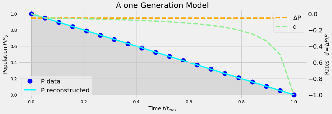
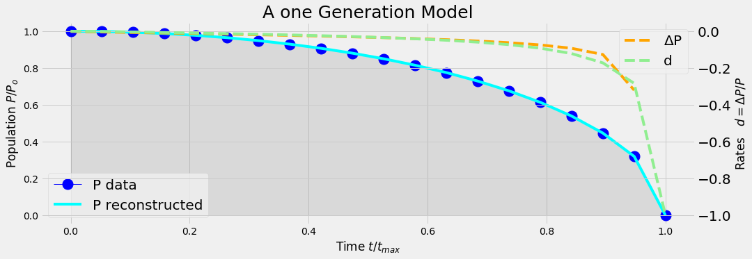
        plt.title('A one Generation Model',  fontsize=25) 
        ax1.legend(loc=3,prop={'size': 20})
        ax2.legend(loc=1,prop={'size': 20})
        plt.show()

We generate 2 data sets of a generation,

(A) the generation diminishes linearly with time
(B) the generation diminishes as a quadratic function of time

def set_generation(case,t):
    if case=='A': a = 1;   b = -1; P = a + b*t;
    if case=='B': a = 1;   b = 1; R = 1; P =  np.sqrt(R**2 - a*t**2)/b
    return P

We simply

compute the death rate
re-construct the time series of the generation again

def analyticModel(case,nt):
    #--- generate population data ---------------
    t = np.linspace(0,1,nt) 
    P = set_generation(case,t)
    #--- compute the death rate ---------------
    dP = np.diff(P)
    d = np.concatenate(([0],dP/P[0:-1]), axis=0)
    #--- reconstruct the time series of the generation ---
    Prec = np.cumprod(1+d)
    #--- plot the result ----------------------
    plot_pop(P,Prec,dP,d,t)

analyticModel('A',20)

png

analyticModel('B',20)

png

Conclusion

Even when the generation diminishes linearly with time, the time series of the death rate is some exponential function of time.

Numerical schemas for integration over time

Several discretization schemes exist for solving numerically an ODE (ordinary differential equation) of the type

$$ \dot{P} = d \cdot P $$

Here only the temporal term $\dot{P} = \frac{dP}{dt}$ has to be considerd (since no derivatives in space are existent). Without going into the details we scetch the following 3 types

forward Euler schema
backward Euler schema
Crank Nicolson schema (generalized as \theta -schema)
....and there are more sophisticated schemas not mentioned here

Each discretization schema is an approximation only to the original ODE. It depends on the type of application which one the best suited is.

A. Forward Euler schema or explicit schema

$$ \frac{P^{n+1}-P^n}{t^{n+1}-t^n} = d \cdot P^n $$

Asuming a constant time step $\Delta t = t^{n+1}-t^n$ we can solve for $P^{n+1}$:

$$ P^{n+1} = P^n (1+d^n\Delta t) $$

B. Backward Euler schema or implicit schema

$$ \frac{P^{n+1}-P^n}{\Delta t} = d^{n+1} \cdot P^{n+1} $$

$$ P^{n+1} = \frac{1}{1-d^{n+1}\Delta t} P^n $$

C. Crank Nicolson schema or $\theta$-schema

The temporal term $\dot{P} = \frac{dP}{dt}$ is a derivative. Its slope is perfectely described by the discretized form $(P^{n+1}-P^n)/(t^{n+1}-t^n)$. But this slope is valid between $P^{n+1}$ and $P^n$, not necessarily however at its endpoints $P^{n+1}$ or $P^n$. An obvious approach is to evaluate the right hand side of the ODE ($d\cdot P$) inbewteen too, e.g. at $d^{n+\frac{1}{2}}P^{n+\frac{1}{2}}$. The generalized $\theta$-schema allows to switch seamlessly between the explicit and implicit schema. With $\theta=\frac{1}{2}$ its called Crank Nicolson schema.

$$ \frac{P^{n+1}-P^n}{\Delta t} = (1-\theta)\:d^{n} P^{n} + \theta\: d^{n+1}P^{n+1} $$

$$ P^{n+1} = \frac{1+(1-\theta)d^n\Delta t}{1-\theta\:d^{n+1}\Delta t} P^n $$

D. Implementation of the 3 numerical ODE solvers

Numerical solvers sometimes need a finer resolution than the data are given. An implementaion has to be prepared to interpolate the parameters given as data. In the following section

we generate the distribution of the population (=times series of a generation)
we derive the death rate
we interpolate the data to the resolution given by the timestep of integration
we solve the ODE by the explicit, the implicit and the Crank Nicolson schema

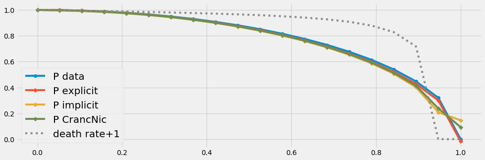
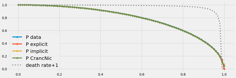
Main results

Even with few data (n=100) all three solvers produce the same results.
If we have very few data (n=20) only the explicit schema is acurate for this (smooth) type of problem. The discretization errors due to very few data points affect the solution of the solvers with an implicit part. This problem vanishes with an increased number of data points.

def threeSolvers(nt,NT):
    #--- generate population data ---------------
    #nt = 20
    t = np.linspace(0,1,nt) 
    P = set_generation('B',t)

    #--- compute the death rate ---------------
    dP = np.diff(P)
    d = np.concatenate((dP/P[0:-1],[-1]), axis=0)

    #--- initialize the solution arrays ---
    #NT = 20
    tt = np.linspace(0, 1, NT)
    qe = np.zeros_like(tt)
    qi = np.zeros_like(tt)
    qc = np.zeros_like(tt)

    dri = sp.interpolate.interp1d(t, d, kind='cubic')
    Dt = np.diff(tt)[0]*NT
    theta = 0.5
    qe[0] = 1.0; qi[0] = 1.0; qc[0] = 1.0;

    for ji,tv in enumerate(tt[1:]):
        ti = ji+1
        fExplicit =      Dt*dri(tt[ti-1])+1
        fImplicit = (1-Dt*dri(tt[ti  ]))**-1
        fCrancNic =  ((1-theta)*Dt*dri(tt[ti-1])+1) / (1-theta*Dt*dri(tt[ti  ]))

        qe[ti] = qe[ti-1] * fExplicit
        qi[ti] = qe[ti-1] * fImplicit
        qc[ti] = qe[ti-1] * fCrancNic

    with plt.style.context('fivethirtyeight'): 
        fig = plt.figure(figsize=(15,5))
        ax1= fig.add_subplot(1, 1, 1)
        plt.plot(t,P,'o-', label='P data')
        plt.plot(tt, qe, 'D-', label='P explicit')
        plt.plot(tt, qi, 'D-', label='P implicit')
        plt.plot(tt, qc, 'D-', label='P CrancNic')
        plt.plot(tt, dri(tt)+1, ':', label='death rate+1')
        plt.legend(loc=3,prop={'size': 20})
        plt.show()

The death rate has to be negativ [0 .. -1] due to our mathematical framework. In order to simplify the graphical implementation we plot $(death rate + 1)$ in the following graphics.

threeSolvers(20,20)

png

threeSolvers(100,100)

png

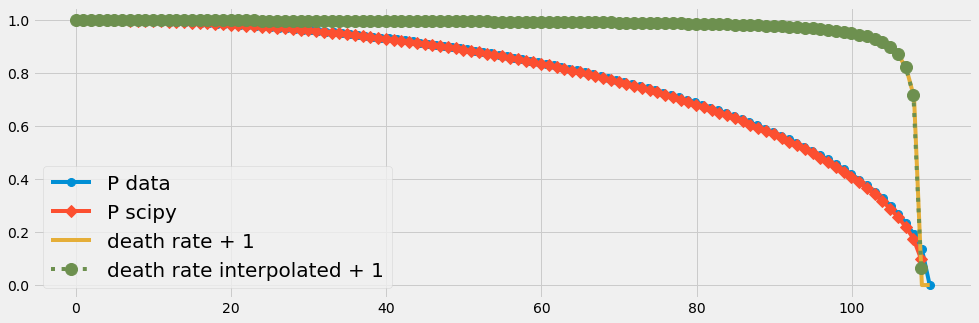
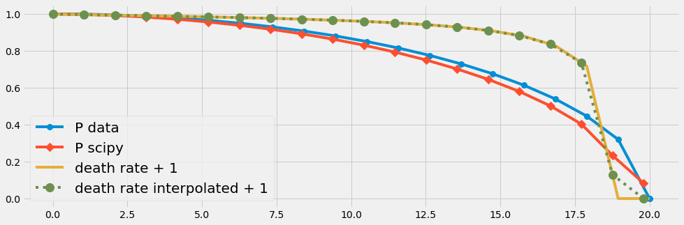
E. Numerical ODE solution with scipy

We try now the ODE solver of scipy in an arangement with temporal changing parameters. We will see again that

the discretization error due to few input data (n=20) affects the numrical solution.
This problem vanishes with an increased number of data points.

def scipySolver(nt,NT):
    #--- generate population data ---------------
    t0 = np.linspace(0,1,nt)
    t = nt*t0
    P = set_generation('B',t0)

    #--- compute the death rate ---------------
    dP = np.diff(P)
    d = np.concatenate((dP/P[0:-1],[-1]), axis=0)

    #--- prepare the interpolation of the death rate
    tt0 = np.linspace(0, 0.99, NT)
    tt = tt0*nt
    dri = interpolate.interp1d(t, d)

    #--- the ODE to solve ----
    def func(x, t, dr):
        return x*dri(t)

    #--- inital conditin and solver ------
    y0 = 1
    args = (dri,)
    y = sp.integrate.odeint(func, y0, tt ,args)

    #--- grafics ------
    with plt.style.context('fivethirtyeight'): 
        fig = plt.figure(figsize=(15,5))
        ax1= fig.add_subplot(1, 1, 1)
        plt.plot(t,P,'o-', ms=8, label='P data')
        plt.plot(tt, y, 'D-', ms=8,label='P scipy')
        plt.plot(t,d+1, '-', label='death rate + 1')
        plt.plot(tt, dri(tt)+1, 'o:', label='death rate interpolated + 1', ms=12)
        plt.legend(loc=3,prop={'size': 20})
        plt.show()

scipySolver(20,20)

png

scipySolver(110,110)

png

HealthyNumerics

Time-dependent integration of a one-generation model