- So 06 August 2017
- MetaAnalysis
- Peter Schuhmacher
- #Bootstrapping, #Monte Carlo, #numerical analysis, #Python
Introduction
Bootstrapping is a useful tool when we have data describing a distribution, but we do not know the type of the distribution and so we do not know how to find out, e.g., confidence values for the mean.
Bootstrapping is part of the Monte Carlo methods and is a numerical method. That means that there is no closed analytic formula to compute the result. The solution is successively approximated by an algorithm that is iterated many times by a computer. In the case of bootstrapping the algorithm builds by random choice a (random) sample of the given data set and computes the arithmetic mean. This is repeated many times and the mean of the means is the estimate for the mean of the data set.
The underlying asumption is that samples behaves toward the data set in the same manner as the data set behaves toward the population. It's a non trivial task of numerical mathematics to proof that this procedure converges toward the desired solution.
Data generation
In this part we generate some data. If we use some known distributions we can check the effectiveness of bootstrapping.
import numpy as np
import scipy.stats as st
float_formatter = lambda x: "%6.2f" % x
np.set_printoptions(formatter={'float_kind':float_formatter})
import matplotlib.pyplot as plt
import matplotlib.colors as mclr
import matplotlib.gridspec as gridspec
def generate_data(case,md,μ=None,σ=None):
    if μ==None: μ = 0.0
    if σ==None: σ = 1.0

    if case=='normal':
        return np.random.normal(μ, σ, size=(md)), st.norm(μ,σ)

    if case=='gamma':
        return np.random.gamma(μ, size=(md)), st.gamma(μ)

    if case=='exponential':
        return np.random.exponential(μ, size=(md)), st.expon(μ)
Estimate of the mean by bootstrapping
bootstrap_mean is an explicit Python program for bootstrapping. (There are also self-contained Python libraries)
- We build a random set of indices (
random_inidices) to build a random sample of the data. - From this random sample we build the mean and store it in an array (
sampleMeans[i]). - The mean of this array (
sampleMeans) is the final result of bootstrapping. - The standrad deviation of
sampleMeansis a bootstrapped estimate of the SE of the sample statistic. - The 2.5- and 97.5-percentiles gives the confidential intervall CI
short_version is a more compact code producing the same as bootstrap_mean .
def bootstrap_mean(data,nRuns):
    nd = len(data)
    sampleMeans = np.zeros(nRuns)
    for i in range(nRuns):
        iLow=0; iHi=nd
        random_inidices = np.random.randint(iLow,iHi, size=nd)
        sample = data[random_inidices]
        sampleMeans[i] = sample.mean()
    return sampleMeans

def short_version(data,nRuns):
    samples = np.array([np.random.choice(data, nd, replace = True) for _ in range(nRuns)])
    return np.mean(samples, axis=1)
Now let's try out this function. You can change the length of the data set nd and how many samples of the data are to be drawn nRuns.
nd=100;
data, rv = generate_data('gamma',nd, μ=2,σ=1)

nRuns = 1000
sampleMeans = bootstrap_mean(data,nRuns)
#sampleMeans = short_version(data,nRuns)
Evaluation and graphical display
μ = sampleMeans.mean()
σ = sampleMeans.std()
CIl, CIu = np.percentile(sampleMeans, [2.5, 97.5])
ydata = rv.pdf(data)
x = np.linspace(rv.ppf(0.001), rv.ppf(0.999),300)
markerSize = 200
print("dataMean bootstrapping : {0:9.4f}".format(μ))
print("standard deviation of the mean: {0:9.4f}".format(σ))
print("CI [2.5, 97.5] : [{0:8.4f},{1:8.4f}]".format(CIl, CIu))
print("dataMean arithmetic : {0:9.4f}".format(data.mean()))
print("deltaM : {0:9.4f}".format(data.mean() - μ ))
print()
#--- Grafics -----------------------------------------------------
figX = 15; figY = 15
fig = plt.subplots(figsize=(figX, figY))
gs = gridspec.GridSpec(2, 2,width_ratios=[1,1],height_ratios=[1,1])
ipic = 0; ax = plt.subplot(gs[ipic])
ax.plot(x,rv.pdf(x),'--k')
ax.scatter(data, ydata, s=markerSize, c='gold', alpha=0.5, edgecolor='g', lw = 2)
ax.axvline(μ, linewidth=4, color='r')
plt.xlabel("values of data points")
plt.ylabel("probability density")
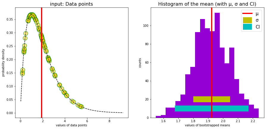
plt.title("input: random Data points", fontsize=16)
ipic = 1; ax = plt.subplot(gs[ipic])
ax.hist(sampleMeans, bins='auto', color='darkviolet') # arguments are passed to np.histogram
ax.hlines(20.0, μ-σ, μ+σ, colors='y', lw=20, linestyles='solid', label='σ')
ax.hlines(10.0, CIl, CIu, colors='c', lw=20, linestyles='solid', label='CI')
ax.axvline(μ, linewidth=4, color='r',label='μ')
plt.xlabel("values of bootstrapped means")
plt.ylabel("counts")
plt.title("Histogram of the mean (with μ, σ and CI)", fontsize=16)
ax.legend(frameon=True,loc='upper right',prop={'size': 15})
plt.show()
dataMean bootstrapping        :    1.9245
standard deviation of the mean:    0.1239
CI [2.5, 97.5]                : [  1.6757,  2.1722]
dataMean arithmetic           :    1.9300
deltaM                        :    0.0054
A note to the confidential interval CI
Under the assumptions of traditional frequentist's statistics the CI does not mean that the interval has a chance of 95% to contain true parameter μ. It means rather that in case we calculate from (infinite) many samples the CI, that 95% of these CIs contain the real parameter μ of the population.
The influence of the number of samples
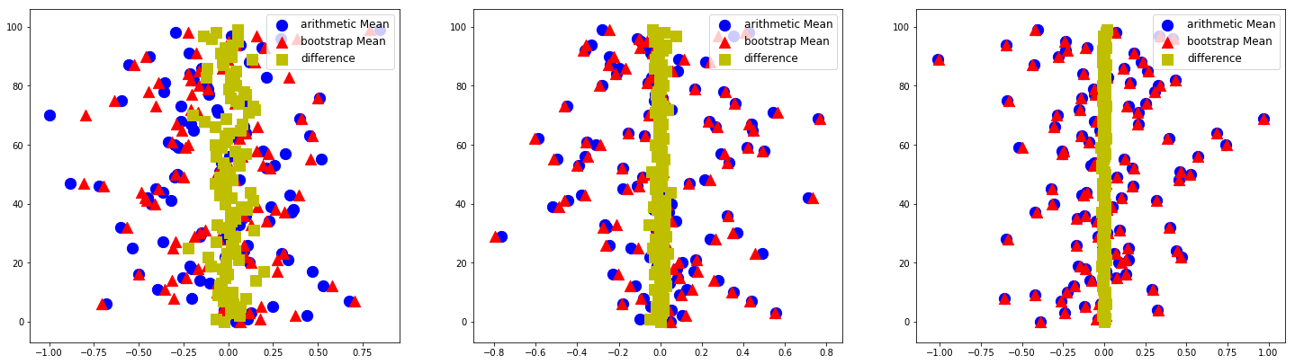
We repeat the whole bootstrapping experiment nRepeat times and generate each time a new data set of length nd=10. For each data set we compute and plot the arithmetic mean (blue points), the bootstrap mean (red points) and the difference between them (yellow points). In a graphic we see nRepeat = 100 such experiments.
We run 3 sets in this manner with the number of bootstraping samples nRuns being 20, 200, and 2000. We can see that the differences (yellow points) converge to zero with increasing number of randomly drwan samples nRuns
def plot_2D(ax,xM,xB,yk):
    ax.scatter(xM,yk, s=150, color = 'b',label='arithmetic Mean')
    ax.scatter(xB,yk, s=150, color = 'r', marker = '^',label='bootstrap Mean')
    ax.scatter(xM-xB,yk, s=150, color = 'y', marker = 's',label='difference')
    ax.legend(frameon=True,loc='upper right',prop={'size': 12})

def run_bootstrapping(nRepeat,nd,nRuns):
    yk = np.zeros(nRepeat)
    xM = np.zeros(nRepeat)
    xB = np.zeros(nRepeat)

    for k in range(nRepeat):
        data, rv = generate_data('normal',nd,μ=0,σ=1)
        sampleMeans = short_version(data,nRuns)
        yk[k] = k
        xM[k] = data.mean()
        xB[k] = sampleMeans.mean()
    plot_2D(ax,xM,xB,yk)
figX = 25; figY = 15
fig = plt.subplots(figsize=(figX, figY))
gs = gridspec.GridSpec(2, 3,width_ratios=[1,1,1],height_ratios=[1,1])

nRepeat = 100; nd=10;

ipic = 0;    ax = plt.subplot(gs[ipic])
nRuns = 20;  run_bootstrapping(nRepeat,nd,nRuns)

ipic = 1;    ax = plt.subplot(gs[ipic])
nRuns = 200; run_bootstrapping(nRepeat,nd,nRuns)

ipic = 2;    ax = plt.subplot(gs[ipic])
nRuns = 2000;run_bootstrapping(nRepeat,nd,nRuns)

plt.show()