Introduction

Monte Carlo methods are probablistic computational techniques. In the core a Monte Carlo algorithm depicts randomly certain values from the value space of a parameter under consideration. Combining several parameters allows to draw stochastic conclusions of relationships. The integration of mathematical functions of the form

gives a certain insight how the Monte Carlo method works.

In oder to perform an integration we want to know how the randomly selected values are distributed: which of the values are equal or smaller than the value of the function and which ones are greater. This is a binary decision that divides the random values in two groups. From the ratio of the size of the groups we can draw our conclusions.

We use the function (= integrand) as a decision criteria only. The algorithm delivers us nothing else than counts/frequencies. The probalistic closure is then:

The area \(A_{below\;function}\) is the unknown area we are interested in. For \(A_{total\;area}\) we choose arbitrary a simple region those area we can compute without difficulties.

Example: determination of \(\pi\)

As an example we choose a circle whose mathematical function is given by the first or the second line:

For the estimate of \(\pi\) the area of the circle is compared with the area of the square 2R by 2R, This ratio is \(\pi/4\):

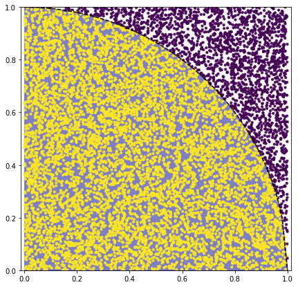
We randomly generate \((x_p,y_p)\)-points. For each point we have to decide wether it is inside or outside the circle. For that we use the difference \(y_p - f(x)\), where \(f(x) = \sqrt{R^2 - x^2}\) is the function for a circle in the first quadrant. We can count how many points are inside the circle. The ratio \(n/N\) is assumed to be equal to the ratio \(A_{circle}/A_{square}\)

Python code

In contrast to the explanation, the python code needs just 6 lines. The number of trials N should be choosen rather 100'000 than 10'000 (which we used to make the grafical display "readeble")

import numpy as np
import matplotlib.pyplot as plt

def f(x): return np.sqrt(1-x*x)  # function for a circle

N = 10000   # number of trials
np.random.seed(2)
x = np.random.rand(N)
y = np.random.rand(N)
n = np.sum( y - f(x) < 0.0) #number of points in the circle


#----- Output and Graphics -------------------
print('PI numpy       : ', np.pi)
print('PI monte carlo : ', 4*n/N)
print('difference     : ', 4*n/(N) - np.pi)

xp = np.linspace(0,1,50)
colors = (np.sign(f(x)-y)+1)/2
area = 10
fig, ax = plt.subplots(figsize=(7, 7))
plt.subplot(111)
plt.plot(xp,f(xp),'--k')
plt.fill_between(xp, f(xp), color='darkblue', alpha=0.5 )
plt.scatter(x, y, s=area, c=colors, alpha=0.9)
plt.axis('equal')
plt.axis([0.0, 1.0, 0.0, 1.0])
plt.show()

PI numpy       :  3.141592653589793
PI monte carlo :  3.1436
difference     :  0.00200734641021