- Di 15 August 2017
- MetaAnalysis
- Peter Schuhmacher
- #Regression, #Monte Carlo, #numerical analysis, #Python, #PyMC
We perfom a linear regression using a Monte Carlo Method which is implemented by the Python library PyMC.
import numpy as np
import pandas as pd
from __future__ import division
import matplotlib.pyplot as plt
%matplotlib inline
%precision 4
plt.style.use('ggplot')
import seaborn as sns
np.random.seed(1234)
import pymc3 as pm
import scipy.stats as st
The MC model
The argument ('y ~ x', data) tells the Monte Carlo Model that a linear relation y ~ x has to be built with data. NUTS is the type of MC-process to proceed the numerical evalutaion. We run the model for 2000 iterations.
#---- generate data -----
n  = 11
aa = 6;   bb = 2
x = np.linspace(0, 1, n)
y = aa*x + bb + np.random.randn(n)
data = dict(x=x, y=y)

#--- set up and run MC-model -----
with pm.Model() as model:
    pm.glm.glm('y ~ x', data)
    step = pm.NUTS()
    trace = pm.sample(2000, step, progressbar=True)
100%|█████████████████████████████████████████████████████████████████████████████| 2000/2000 [00:13<00:00, 146.45it/s]
Evaluation
If we take the Maximal Probability (MAP) as final result for slope and intercept, then there are no diffrences to the same paramteres computed by scipy or numpy procedures. The statistics of the MC ouput is given below.
#---evaluate the results -------
map_estimate = pm.find_MAP(model=model);
print('--------------------------------------------------------------------------')
print('MC MAP_estimate:\n', pd.Series(map_estimate))

#---- compare with linear regression done by scipy and numpy
from scipy.optimize import curve_fit
def func(x, a, b):  return a * x + b
popt, pcov                                  = curve_fit(func, x, y)
slope, intercept, r_value, p_value, std_err = st.linregress(x,y)
f_poly                                      = np.polyfit(x, y, 1)

#---- print output ----------------
print('--------------------------------------------------------------------------')
print('scipy lingress: slope, intercetp, R2 : ',slope, intercept,r_value**2)
print('scipy curvefit : ', popt)
print('numpy polyfit  : ', f_poly)
print('--------------------------------------------------------------------------')
pm.summary(trace)
Optimization terminated successfully.
Current function value: 48.431842
Iterations: 15
Function evaluations: 19
Gradient evaluations: 19
--------------------------------------------------------------------------
MC MAP_estimate:
Intercept 2.161765243874408
sd_log_ 0.10758781873613464
x 5.62432432188842
dtype: object
--------------------------------------------------------------------------
scipy lingress: slope, intercetp, R2 : 5.62432435532 2.16176516782 0.736780992063
scipy curvefit : [ 5.6243 2.1618]
numpy polyfit : [ 5.6243 2.1618]
--------------------------------------------------------------------------
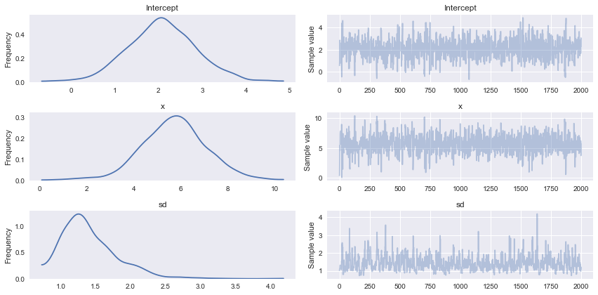
Intercept:
Mean SD MC Error 95% HPD interval
-------------------------------------------------------------------
2.081 0.821 0.027 [0.506, 3.740]
Posterior quantiles:
2.5 25 50 75 97.5
|--------------|==============|==============|--------------|
0.496 1.564 2.070 2.595 3.734
x:
Mean SD MC Error 95% HPD interval
-------------------------------------------------------------------
5.719 1.427 0.045 [3.003, 8.672]
Posterior quantiles:
2.5 25 50 75 97.5
|--------------|==============|==============|--------------|
2.782 4.848 5.748 6.582 8.501
sd:
Mean SD MC Error 95% HPD interval
-------------------------------------------------------------------
1.418 0.407 0.021 [0.777, 2.202]
Posterior quantiles:
2.5 25 50 75 97.5
|--------------|==============|==============|--------------|
0.838 1.139 1.339 1.622 2.356
Grafical ouput
The grafical output displays the probability distributions of the output parameters.
#---- graphical display ----------------
AA = map_estimate['x']
BB = map_estimate['Intercept']
pm.traceplot(trace);
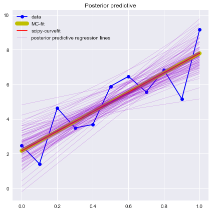
plt.figure(figsize=(7, 7))
plt.plot(x, y, 'b-o', label='data')
plt.plot(x, func(x, AA, BB),'y-', lw=8,label='MC-fit')
plt.plot(x, func(x, *popt), 'r-', label='scipy-curvefit')
pm.glm.plot_posterior_predictive(trace, samples=100,
label='posterior predictive regression lines',
c='darkviolet', alpha=0.95)
plt.legend(loc='best');
plt.show()