To make as few assumptions as possible is - among other - one motivation to use numerical methods in statistics. If you find some empirical distribution from your problem under consideration, you may be faced with the question how to use this distribution as a sampling engine. This is not too difficult, and we give an example here.

import numpy as np
import pandas as pd
import matplotlib.pyplot as plt
import matplotlib.colors as mclr

Data generation

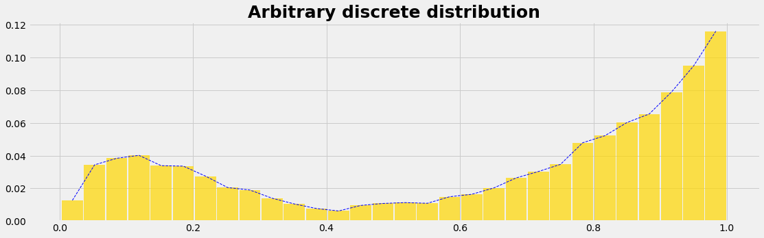
We use the beta distribution to generate some arbitrary looking distribution. With different paramters we generate 2 arrays, which we concatenate to one data set of a population. So we have now a distribution that is

• empirical
• discrete (given by data points)
• the analytical function is unknown
• the inverse function is unknown too

prev = 0.7
NP = 10000
nI =  round(NP*prev)
nH = NP-nI

#--- generate the data ---
value_h = np.random.beta(2, 9, nH)
value_i = np.random.beta(5, 1, nI)
value_c = np.concatenate((value_h, value_i))

#--- analyse the data, compute the middle of the data classes (bins)---
nBins=30
count_c, bins_c, = np.histogram(value_c, bins=nBins)
myPDF = count_c/np.sum(count_c)
dxc = np.diff(bins_c)[0];   xc = bins_c[0:-1] + 0.5*dxc

plot_distrib1(xc,myPDF);

Sampling

If we want a random number generator that returns data with the distribution of our empirical distribution we can achieve that in 3 steps:

1. we need the cumulative distribution function (CDF, also cumulative density function) of our empirical distribution.
2. as driving engine we need from our computer the uniform random generator that gives data in the interval [0, 1], which is the value range of the CDF (and which is the y-axis of the CDF-graph)
3. we have to identify to which element of the CDF the random number fits best and we have to count this hit (this is the transformation to the x-axis)

One can imagine that the uniform random numbers are sun rays that are emitted from the y-axis on the left and travel to the right to the CDF-curve. The CDF-curve can be interpreted as a hill which get's more solar energy on the steeper parts and less on the flater parts due to the inclination. The resulting energy profil will be a data set distributed as the PDF of our empirical distribution.

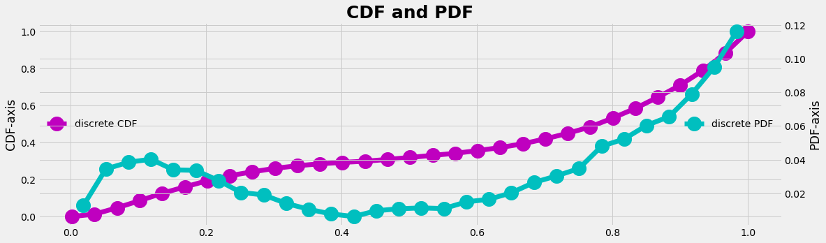
The CDF can be found as the cumulative sum of our empirical PDF distribution.

#--- compute the CDF ----
myCDF = np.zeros_like(bins_c)
myCDF[1:] = np.cumsum(myPDF)
plot_line(bins_c,myCDF,xc,myPDF)

Our random number generator

In the follow code we run with the for-loop nRuns examples and count the hits in the X-array. In the code lines inbetween we find out to which data-element of the CDF an emitted unit random number fits best. For that, we pick out the location in the CDF-array where the random number is the first time larger than the CDF-value. Then we round to the closer element. This generator is designed for discrete values. For continous values a slightly different algorithm may be designed.

def get_sampled_element():
    a = np.random.uniform(0, 1)
    return np.argmax(myCDF>=a)-1

def run_sampling(myCDF, nRuns=5000):
    X = np.zeros_like(myPDF,dtype=int)
    for k in np.arange(nRuns):
        X[get_sampled_element()] += 1
    return X/np.sum(X)

X = run_sampling(myCDF)

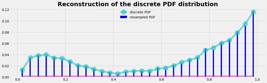
The result

As a result we are able to reconstruct the PDF of the empirical distribution with our random number generator using myCDF as input.

plot_distrib3(X)

Python code: graphics

def plot_distrib1(xc,count_c):
    with plt.style.context('fivethirtyeight'): 
        plt.figure(figsize=(17,5))
        plt.plot(xc,count_c, ls='--', lw=1, c='b')
        wi = np.diff(xc)[0]*0.95
        plt.bar (xc, count_c, color='gold', width=wi, alpha=0.7, label='Histogram of data')
        plt.title('Arbitrary discrete distribution', fontsize=25, fontweight='bold')
        plt.show()
    return

def plot_line(X,Y,x,y):
    with plt.style.context('fivethirtyeight'):
        fig, ax1 = plt.subplots(figsize=(17,5))
        ax1.plot(X,Y, 'mo-', lw=7, label='discrete CDF', ms=20)
        ax1.legend(loc=6, frameon=False)
        ax2 = ax1.twinx()
        ax2.plot(x,y, 'co-', lw=7, label='discrete PDF', ms=20)
        ax2.legend(loc=7, frameon=False)
        ax1.set_ylabel('CDF-axis');  ax2.set_ylabel('PDF-axis'); 
        plt.title('CDF and PDF', fontsize=25, fontweight='bold')       
        plt.show()   

def plot_distrib3(X):
    with plt.style.context('fivethirtyeight'): 
        plt.figure(figsize=(17,5))     
        plt.bar(xc, X ,color='blue', width=0.005, label='resampled PDF')
        plt.plot(xc, np.zeros_like(X) ,color='magenta', ls='-',lw=13, alpha=0.6)
        plt.plot(xc,myPDF, 'co-', lw=7, label='discrete PDF', ms=20, alpha=0.5)
        plt.title('Reconstruction of the discrete PDF distribution', fontsize=25, fontweight='bold')
        plt.legend(loc='upper center', frameon=False)
        plt.show()