A toy example of a diagnostic test

The performance of the diagnostic test in clinical evaluation

Let's assume a diagnostice test detects correctely 90% of the those cases that are ill, and rules out correctely 95% of the cases that are not ill. Let's further assume that 2% of the population are affected by this illness. So we have:

Prevalence of the illness: 0.02
Sensitivity of the diagnostic test: 0.90
Specificity of the diagnostic test: 0.95

This sounds pretty good !

The performance of the diagnostic test in medical practice

To make things easier let's consider an arithmetic example with a population of 1000 peoples.

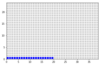
Prevalence:

population 1000 peoples
20 are ill (0.02*1000 = 20)
980 are healthy (1000-20 = 980)

z[0:int(nIll),0] = 1
plot_table(x,y,z)

png

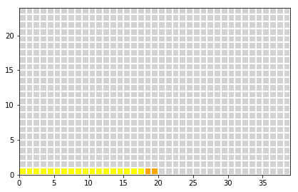
Sensitivity:

90% of the ill peoples = 0.90*20 = 18 are detected correctely (true positive)
10% of the ill peoples = 0.01*20 = 2 are not detetced (false negative)

z[0:int(truePositive),0] = 2
z[int(truePositive):int(nIll),0] = 3
plot_table(x,y,z)

png

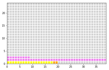
Specificity:

95% of the healty peoples = 0.95*980 = 931 are classified as healthy (true negative)
5% of the healty peoples = 0.05*980 = 49 are classidied as ill (false positive)

z[0:int(falsePositive),1] = 4
z[0:int(falsePositive-nx),2] = 4
plot_table(x,y,z)

png

Result for the positive tests:

among the positive tests are 18 correct and 49 wrong
in medical practice 18/(18+49) = 27% of the positive tests are right (positive prediction value)
in medical practice 49/(18+49) = 73% of the positive tests are wrong

Example: Breast cancer screening

Typical parameters:

Prevalence of breast cancer at age of 40: ~0.01
Sensitivity of mammography: ~0.80
Specificity of mammography: ~0.90

Benefit

assume 1000 women are screened by mammography
8 women are identified correctely as suffering from breast cancer
The positive predictive value is 7.4%

Harm

99 women are identified as being ill despite they are healthy

Without utility

2 women are not identified as being ill despite they are ill
891 healthy women are screened and identified as being healthy

dfB

	ill	healthy	Σ tests
positive	8.0	99.0	107.0
negative	2.0	891.0	893.0
Σ states	10.0	990.0	1000.0

Mammography.get_summary(C)

7.476636     % of the positive tests are right (positive pr...
92.523364    % of the positive tests are wrong (false posit...
dtype: object

Some conclusions

Reasoning about the screening strategy

with a low prevalence of ~0.1 the size of the groups (healthy group, ill group) is very unevenley distributed
as a consequence the rate of true positive cases is low, and the rate of false positive cases is high
a thorough screnning (100%) is on one side costy and with a positive detective rate of 7.4% not efficient. On the other side it brings harm to the false postive identified women (unnecessary biospy, psychological pressure e.g.)
one might think about different screenings strategies. From the statistical point of view approaches seem to be interesting that are able to reduce the rather large number of unnecessary screened peoples, a two level test e.g., that builds in a first step a smaller group of peoples with a higher risk of the desease under consideration.

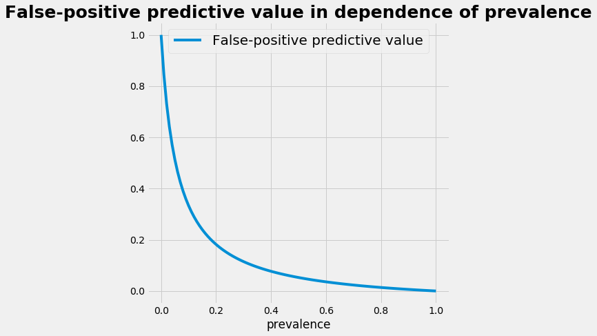
The influence of the prevalence

with a low prevalence the positive predictive value is small and the false positive predictive value is high
the relation between the prevalence and the positive predictive value is plotted below
statistically speaking: building a smaller subgroup that contains the potential patients raises the prevalence in the subgroup. This raises the efficency of the application of a diagostic test.

plot_p_ppv()

png

What type of statistic is it ?

Note, that we have got the results just by counting the occurence of the different cases. So we had no philosophical discussions wether it is Frequentist's or Bayesian statistics.
despite of this peace between the methods it's worth to mention that there is an aspect, that is related with the Bayesian formula: it's the change of perspective.
We start with the perspective of the diagnostic test: given a group of persons that ARE ill, what is the ability (= probablilty) of the diagnostic test to detect the disease \(\mathbf{P(test=positive \mid ill)}\).
We end with the patient's perspective: given a test that is positive, what is the probablity that the patient IS ill \(\mathbf{P(ill \mid test=positive)}\)

Python Code: Analysis with the graphical tables

import numpy as np
import pandas as pd
import matplotlib.pyplot as plt
import matplotlib.colors as mclr

def init_table(nx,ny):
    #---- set the 1-dimensional arrays in x- and y-direction
    ix = np.linspace(0,nx-1,nx)
    iy = np.linspace(0,ny-1,ny)

    #---- use the outer product of 2 vectors -----------
    x = np.outer(ix,np.ones_like(iy))  # X = ix.T * ones(iy)
    y = np.outer(np.ones_like(ix),iy)  # Y = ones(ix) * iy.T
    z = np.zeros_like(x) 
    return x,y,z

def plot_table(x,y,z):
    fig = plt.figure(figsize=(15,6)) 
    myCmap = mclr.ListedColormap(['lightgrey','blue', 'yellow','orange','violet', 'lightgrey'])
    ax4 = fig.add_subplot(121)
    ax4.pcolormesh(x, y, z, edgecolors='w', lw=1, cmap=myCmap)
    ax4.set_aspect('equal')
    plt.show()

nx = 40; ny = 25
Np = nx * ny
prev = 0.02
sens = 0.90
spec = 0.95

nIll = Np*prev
nHealthy = Np*(1-prev)

truePositive = nIll * sens;     falseNegative = nIll*(1-sens)
trueNegative = nHealthy * spec; falsePositive = nHealthy * (1-spec)

sumPositive = truePositive+falsePositive
sumNegative = falseNegative+trueNegative

PC_TruePos =  truePositive/sumPositive
PC_FalsePos = falsePositive/sumPositive

PC_TrueNeg =  trueNegative/sumNegative
PC_FalseNeg = falseNegative/sumNegative

x,y,z = init_table(nx,ny)
z[-2,-2]=5

Python Code: Analysis of the diagnostic test with a Python class

class DiagnosticAnalysis:
    def __init__(self,Np,prev,sens,spec):
        self.Np = Np       #size of population
        self.prev = prev   #prevalence
        self.sens = sens   #sensitiviy
        self.spec = spec   #specitivity

    def get_df(self,Data):
        columns = np.array(['ill', 'healthy','Σ tests'])
        index   = np.array(['positive', 'negative','Σ states'])
        df = pd.DataFrame(data=Data, index=index, columns=columns)     
        return df

    def ContingencyTable(self):
        nIll = self.Np*self.prev
        nHealthy = self.Np*(1-self.prev)

        truePositive = nIll * self.sens;     falseNegative = nIll*(1-self.sens)
        trueNegative = nHealthy * self.spec; falsePositive = nHealthy * (1-self.spec)

        sumPositive = truePositive+falsePositive
        sumNegative = falseNegative+trueNegative

        nData = np.array([['true Positive',' false Positive', 'sum Positive'], 
                          ['false Negative', 'true Negative', 'sum Negative'],
                          ['nIll', 'nHealthy', 'Np']])  
        dData = np.array([[truePositive, falsePositive, sumPositive], 
                          [falseNegative, trueNegative, sumNegative],
                          [nIll, nHealthy, self.Np]])
        rData = dData/self.Np
        #print(nData);print(dData);print(rData)
        return nData,dData,rData, \
               self.get_df(nData), self.get_df(dData), self.get_df(rData)

    def get_summary(self,D):
        sData = np.array([D[0,0]/D[0,2], D[0,1]/D[0,2]]) *100
        sText = np.array(['% of the positive tests are right (positive prediction value)', 
                          '% of the positive tests are wrong (false positive prediction value)'])  
        return pd.Series(index=sData, data=sText)

Population = 1000.0;  prevalence = 0.01; sensivity = 0.80;   specivity = 0.90
Mammography = DiagnosticAnalysis(Population,prevalence,sensivity,specivity)
A,B,C,dfA,dfB,dfC = Mammography.ContingencyTable()

Mammography.get_summary(C)

7.476636     % of the positive tests are right (positive pr...
92.523364    % of the positive tests are wrong (false posit...
dtype: object

Python Code: Relation between prevalence and positive predictive value

def plot_p_ppv():
    prevalences = np.linspace(0,1,101)
    falsepositives = np.zeros_like(prevalences)
    Population = 1000.0;  prevalence = 0.02; sensivity = 0.90;   specivity = 0.95

    for jj,prevalence in enumerate(prevalences):
        D = DiagnosticAnalysis(Population,prevalence,sensivity,specivity)
        A,B,C,dfA,dfB,dfC = D.ContingencyTable()
        falsepositives[jj] = C[0,1]/C[0,2]

    with plt.style.context('fivethirtyeight'):  # 'fivethirtyeight'
        plt.figure(figsize=(7,7))
        plt.plot(prevalences, falsepositives, label="False-positive predictive value")
        plt.xlabel('prevalence')
        plt.title('False-positive predictive value in dependence of prevalence', fontsize=25, fontweight='bold')
        plt.legend(loc='upper center',prop={'size': 20})
        plt.show()

HealthyNumerics

MetaAnalysis: Screening with a binary diagnostic test