The Monti Hall problem came out of a US TV-game in the 1970's and got wide publicity about problem solving statistically. It's about the role of the participant at the TV-game and some external statistical experts which gave advisory what the best gaming strategy is. You can transfer it easely to medical research and seeking a strategy that proofs to be the most suitable to reach ceratin aims in healthcare.

The game runs as follows:

there are three closed doors. Behind one door is the main prize, a trendy car, while behind the other two doors are goats.
The participant has two choices to get the prize.
Step 1: The participant may indicate behind which door the prize is (1. choice).
Step 2: The TV-moderator (Monty Hall) is free to open any door and opens a door.
Step 3: The participant is asked by the moderator whether she wants to stay with her first chocie or whether she wants to indicate the other remainig door (2. choice).
Step 3: The moderator opens the indicated door and the participant gets what's behind it.

The question is: what is the best strategy to win the main prize ?

The informational bias

We recommend to run yourself a self test in this order:

scetch what you think to be the best gaming strategy
get some advisory by watching different video clips in YouTube about the Monty Hall problem
get some advisory by reading about the Monty Hall problem in Wikipedia

In YouTube you will see many different hand weaving poeples with hand weaving arguments, augmented with decision trees or Bayesian formulas, explainig very focussed what the correct answer is. If you are not really at home in statistics, I think you will not be really be convinced by any of these contributions but will rather think: "It seems to be complicated with many falling tricks - let statistically talented people do that job". I think that's not the best conclusion you can draw.

Consulting Wikipedia about the Monty Hall problem you will more learn about the history of the story. I'm shure you soon will recognize it's not only about doing the things right but doing the right things first: it's about the statistical model. In the Monti Hall example it's first not obivious and not a common agreement what the appropriate statistical model is, because it's not fixed what game the TV-moderator really plays, leading to different approaches what the best gaming strategy is.

If you imagine that it is not about the behaviour of a TV-moderator but about the behaviour of patients then it's obvious that you should be involved in about what the statistical model is, which is not a mathematical issue but an issue of the real world problem under consideration.

Solving the problem numerically by reconstructing the game

"Numerically" means that we do not seek for a solution by analytical formulas but seek to solve the problem with numbers directely. The workflow is as follows:

We go through the process step by step.

Each step has a certain perspective that gives an information layer. We try to transform this perspective into a mathematical form by using distribution vectors as a describing tool.

We model explicitely what the connection to the next step and information layer is.

In development stage we go through the steps with one randomly choosen possibility (= 1 random walk).

In evaluation stage we run the model many times (random walks) and analyzee the results.

In order to make the generality of the approach visible, we will demonstrate it with 7 doors, but we will run the model with 3 doors only later.

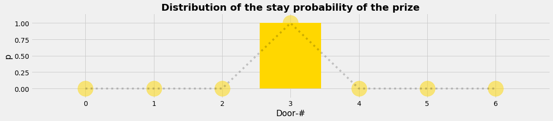
Layer 1: The prize behind the doors

Layer 1 is the perspective of the goats and the prize. We set up the model as what we see in the TV-game: we have nD doors and so we set up a vector (= an array) of length nD and choose randomly behind which door the prize has to be located. The mathematical translation is that we get a stay distribution of the prize which is 1 at the door where the prize is behind and equals zero else.

nD = 7; nP = 1
xnd = np.arange(nD)
L1_PDF = np.r_[np.repeat(1,nP), np.repeat(0,nD-nP)]
np.random.shuffle(L1_PDF)
plot_distr(xnd,L1_PDF,'Distribution of the stay probability of the prize','gold')

png

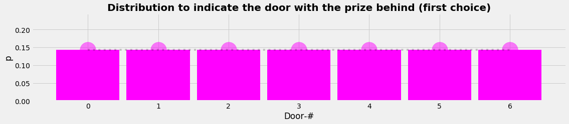
Layer 2: The first choice of the participant

Layer 2 is the participant's perspective. For the participitant is the stay of the prize a hidden layer she has no information about. The model is that she can and has to choose just any door. The mathematical translation is a uniform distribution saying that any door has the same probability to have the prize behind. The process is that randomly a door number is choosen out of the given distribution.

L2_PDF = np.ones(nD)/nD
plot_distr(xnd,L2_PDF,'Distribution to indicate the door with the prize behind (first choice)','magenta')

png

L2_door = np.random.randint(0,nD)
print("Guess 1 is door number ", L2_door)

Guess 1 is door number  1

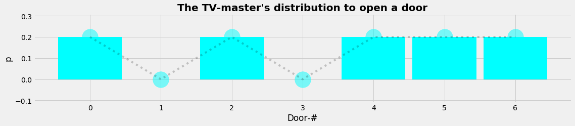
Layer 3: The role of the TV-moderator

Layer 3 is the moderator's perspective. His role is open to discussion. He could be very neutral and just open the door the participant indicates. But it's more obvious that he wants to keep the game exciting. So he does not want to finish the game after the first step already. And he might interessted to generate an atmosphere of emotional uncertainity which he can achieve when he opens any other door but this one the participant has indicated.

We decide to use the following model: The TV-moderator will open any door, but never the door with the prize behind and never the door the participant has guessed. The mathematical translation leads us to a distribution that is uniform execpt at the door with the prize behind and at the door guessed by the participant where the values of the distribution are zero. The process is to draw randomly a 1-element sample from this arbitrary, empirical distribution.

L3_PDF = 1-L1_PDF; L3_PDF[L2_door]=0
L3_PDF = L3_PDF/np.sum(L3_PDF)
plot_distr(xnd,L3_PDF,"The TV-master's distribution to open a door",'cyan')

png

L3_CDF = np.zeros(len(L3_PDF)+1)
L3_CDF[1:] = np.cumsum(L3_PDF)
a = np.random.uniform(0, 1)
L3_door = np.argmax(L3_CDF>=a)-1
print("The TV-moderator opens door ", L3_door)

The TV-moderator opens door  6

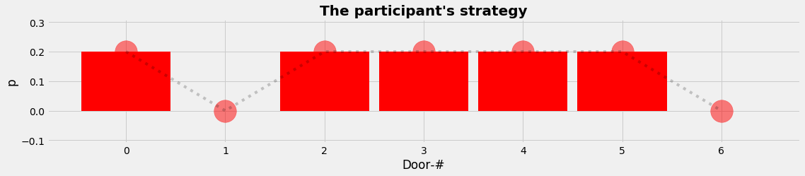
Layer 4: The strategy of the participant for the second choice

Layer 4 is the participant's perspective again. Her strategy is open to discussion too. It is the question how far she anticipates a suspected behaviour of the moderator. So we seek for a model that expresses the parciptant's aim to include the suspected behaviour and to draw some assumed information out of that.

We decide to use the following model: The participant will indicate any door, but never the door that is already open :-) and never the door she has already guessed. The mathematical translation leads us to a distribution that is uniform execpt at the door that is open and at the door guessed by the participant where the values of the distribution are zero. The process is again to draw randomly a 1-element sample from this arbitrary, empirical distribution.

L4_PDF = np.ones_like(L1_PDF); 
L4_PDF[L2_door]=0; L4_PDF[L3_door]=0;
L4_PDF = L4_PDF/np.sum(L4_PDF)
plot_distr(xnd,L4_PDF,"The participant's strategy (second choice)",'red')

png

L4_CDF = np.zeros(len(L4_PDF)+1)
L4_CDF[1:] = np.cumsum(L4_PDF)
a = np.random.uniform(0, 1)
L4_door = np.argmax(L4_CDF>=a)-1
print("The participant indicates door ", L4_door)
if L1_PDF[L4_door] == 1:
     print("...and wins the CAR !!!")
else: print("...and wins a goat")

The participant indicates door  2
...and wins the CAR

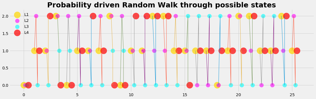
Random walk runs

Each single case and step may be imponderable, but we want to know which strategy is advantageous on the long run. That is exactely what we can do numerically with the computer: We run a long run and repeat the game with many random walks that are controlled by the distributions we have formulated.

With the strategy, formulated by the models above, the participant on the long run will in 66 % of the games win the prize (mean=0.665599, std=0.149588)

plot_run()

png

Lessons to learn

We can draw some conlusions from the Monty Hall model:

This approach links several layers of information / stakeholders / treatment effects / states of patients / etc.
Each layer can be adressed seperately and specified.
Each layer is accessible for
open discussion what the important features are
formulation of an appropriate model
translation into a mathematical form
explict coding of the processes in relation to other layers
evaluation of expected values and uncertainities

The approach is self-contained and works with the data that belongs to the problem under consideration (no foreign distributions from somewhere else)

This approach has some features that are adressed in other model types too:

it is of Markov-type because it is organized around states of patients, populations etc.
it is of Monte Carlo-type because it's driven by an informed random process.
it is of Bayesian-type because it adresses the specific perspective of each stakeholder (layer) under the precondition that the previous layer is given.
it is dynamic because during the walk a layer can adapt its preferred distribution according to the prevailing circumstances

Python code

import numpy as np
import pandas as pd
import matplotlib.pyplot as plt
import matplotlib.colors as mclr

def plot_distr(x,y,title,c):
        with plt.style.context('fivethirtyeight'): 
            plt.figure(figsize=(17,3))
            plt.scatter(x, y, color=c, s=1000, alpha=0.5)
            plt.bar(x, y, width=0.9, color=c)
            plt.plot(x,y,'k:', alpha=0.2)
            plt.xlabel('Door-#'); plt.ylabel('p')
            plt.title(title, fontsize=20, fontweight='bold')
            plt.show()

def random_walk(nD,nP,W):
    xnd = np.arange(nD)
    L1_PDF = np.r_[np.repeat(1,nP), np.repeat(0,nD-nP)]
    np.random.shuffle(L1_PDF)
    L1_door = np.argmax( L1_PDF>=1)

    L2_PDF = np.ones(nD)/nD
    L2_door = np.random.randint(0,nD)

    L3_PDF = 1-L1_PDF; L3_PDF[L2_door]=0
    L3_PDF = L3_PDF/np.sum(L3_PDF)
    L3_CDF = np.zeros(len(L3_PDF)+1)
    L3_CDF[1:] = np.cumsum(L3_PDF)
    a = np.random.uniform(0, 1)
    L3_door = np.argmax(L3_CDF>=a)-1

    L4_PDF = np.ones_like(L1_PDF); 
    L4_PDF[L2_door]=0; L4_PDF[L3_door]=0;
    L4_PDF = L4_PDF/np.sum(L4_PDF)
    L4_CDF = np.zeros(len(L4_PDF)+1)
    L4_CDF[1:] = np.cumsum(L4_PDF)
    a = np.random.uniform(0, 1)
    L4_door = np.argmax(L4_CDF>=a)-1

    if L4_door == L1_door: W[0] += 1
    else: W[1] += 1
    return W , np.array((L1_door,L2_door,L3_door, L4_door))

nSet = 1000
S = np.zeros(nSet)
nD = 3; nP = 1
nRuns = 10;
for j in np.arange(nSet):
    W = np.zeros(2)
    D = np.zeros(4)
    for k in np.arange(nRuns):
        W,P = random_walk(nD,nP,W)
        D = np.vstack( (D, P ))
    S[j] = W[0]/np.sum(W)
print("mean: ",S.mean())
print("std : ",S.std())

mean:  0.6693
std :  0.1488203951076599

kx = np.arange(nRuns+1); 
dx1=0.15; dx2=2*dx1; dx3=3*dx1; dx4=4*dx1;
L1 = D[:,0]; L2 = D[:,1]; L3 = D[:,2]; L4 = D[:,3]

def plot_run():
    with plt.style.context('fivethirtyeight'): 
        plt.figure(figsize=(17,5))     
        plt.scatter(kx,     L1 ,color='gold',   s=500, alpha=0.7, label='L1')
        plt.scatter(kx+dx1, L2 ,color='magenta',s=200, alpha=0.6, label='L2')
        plt.scatter(kx+dx2, L3 ,color='cyan',   s=200, alpha=0.6, label='L3')
        plt.scatter(kx+dx3, L4 ,color='red',    s=500, alpha=0.7, label='L4')        
        for k in kx:
            plt.plot((k,k+dx1,k+dx2,k+dx2),(L1[k],L2[k],L3[k],L4[k]),ls='-',lw=1)
        plt.title('Probability driven Random Walk through possible states', fontsize=25, fontweight='bold')
        plt.legend(loc='best', frameon=False)
        plt.show()

HealthyNumerics

NumericalStats: WHY and HOW to involve medical researchers into the statistical model building