Full disclosure: I hate flipping coin examples. But they they are close to ill or healthy and contain the ingradients to think about how statistics can be done. So let's have a look at this inevitable case study.

1. we explain briefly the tradtional flipping coin example
2. we introduce the use of vectors for that example
3. we give some arguments WHY this can be usefull
4. we give a short outlook how an application might look like for that example

Using points of values for the flipping coin model

• Physics: A tossed coin lands due to its angular momnentum al-al-al-almost never on its edge. So we can approximate the space of state of outcome with two states only: head or tail.
• (In-)Dependency of outcome: The two states are perfectely dependent on each other, perfectely negative correlated. No overlapping areas of outcome: a coin can not land on both of its sides simultaneously, not even a little bit.
• Countability: The outcome is observable. We can count the events without measurement instruments. So we do not need any approximations about what we see.
• The mental model: all these circumstances lead us to conlcusion that the probability (in form of odds) of the side a coin lands after tossing is 50:50. Furthermore, if the probability (in form of odds) is different than 50:50 we are convinced that the coin is wrong or that the tossing person is wrong, not that the model is wrong. This conviction is our mental model.
• The statistical model: We use a tool (Bernoulli distribution, for situations with binary outcome), that counts the events and that tells us something about the probability of certain events after taking all the different possibilities of outcomes into account. The free variable is the number of events with outcome 'head' (or it might be 'tail' too). The probability p that can be found in the formula is not a free variable but an a priori parameter to describe the coin-flipping-model. We will call it later θ.

Lessons to learn from the flipping coins

• Most of the time we would like to know the probablities of interrelations and events that are more interesting than the landing side of a coin.e.g:
• high and low pressure in the atmosphere and its consequences on the weather conditions or
• high and low pressure in the blood vessels and its consequences on the living conditions.
• For this type of problems it would not be a good idea, to be as convinced as with the coin-flipping-model, that rather the world is wrong than our model. So we have to think about carefully how we can take into account all the different uncertainities.
• A modest first step is, that we formally introduce the possibility to include vectors of information (whole distributions e.g.) instead single 'representative' points of information only. We describe that below.

Inverse inference: Find Your hidden layer

• Even when everything seems to be definite and clear around the coin, there is still a hidden layer in the flipping coin experiment.
• You can find it by the question: "If everything is definite and clear around the coin, why is tossing coins a random experiment ?"
• If You are the person that is tossing the coin, then the inverse inference is that You are a randomly acting event. Would You say that is a good model to describe yourself ?

The statistical formula

Using the binomial distribution

then is \(B\) the probability of \(k\) succesful events given \(n\) trials and the probability \(p\) of a singel event.

Let's rename this formula to

• on the left side we suppress the dependence on \(n\) because it is regarded as part of the experimental design that is considered fixed
• \(\theta\) is a model parameter. We can call it bias. It expresses wether one side (#0) or the other side (#1) of the tossed coin is preferred. It is dimensionless and has the range of value \([0..1]\). The value \(\theta = 0.5\) means equally biased which is the same as not biased.
• \(y\) are observational, gathered data.

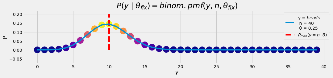
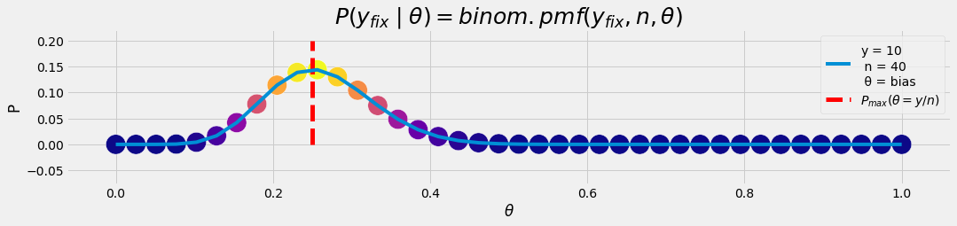
The formula is used ususally in the following manner: What is the probability for y=10 succesful events given n=40 experiments and a bias θ=0.25 ?

• n = 40 experiments
• y = 10 succesful events
• θ = 0.25 bias, model parameter
• \(P\; (y \mid\theta) = 0.144\)

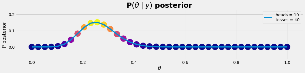
NOTE: most of the time we are interested in \(P(\theta \mid y)\) as a final result rather than in \(P(y\mid \theta)\) .

From value points to distribution vectors

• We can write the observational, gathered data as a vector \(\vec y = (y_0, y_1, ... , y_n)\).
• The same we can do with the model parameter \(\vec θ = (θ_0, θ_1, .., θ_n)\)

With this vectors we have both items, data \(y\) and model parameter \(\theta\), in the calculation schema explicitly. Later we will use this opportunity to fill the vectors with the distributions of \(y\) and \(\theta\). And if we do not know what the appropriate (analytical) distribution is, we will generate numericaly a surrogate out of the data we have.

Using this vectors we have now a 2-dimensional distribution \(P(\vec y, \vec\theta)\) which can vary in both parameters. For the moment we do not fill the vectors with distributions. We discretisize \(\vec y\) and \(\vec\theta\) in \(n\) equidistant points. So what we see on the 2-dimensional graph is a systematic table with the \(P\) values of the binomial distribution.

θ = 0.25   # bias
nToss = 40 # experiment: tossing nToss times
get_likelihood(θ,nToss)
get_pTable(80)

WHY can this be helpful ?

• we are now able to include uncertainities in form of distributions for both items: for the data \(y\) and for the model parameter \(θ\)
• most of the time we are interested in \(P(\theta \mid y)\). That means we have observed data \(y\) (with uncertainities in form of variances) and an idea about a modell \(M(\theta)\) (with uncertainities about the appropriate parameter \(\theta\)) and we want to know up to what degree the data \(y\) and the model \(M(\theta)\) fit together.
• We can include both types of uncertainities throughout the evaluation. When reporting the final result we are able to report the final uncertainities too.
• Often it's not obvious what type of statistical distribution observed data \(y\) do have. In this case we can use numerical sampling methods (bootstrapping, Monte Carlo) to draw samples of the unknown and arbitrary distribution of \(y\).
• This approach makes sense when there is a demand for accuracy and risk handling in the decision making proces.

Opportunities and consequences

• The type of model becomes an explicit part of data modelling and analysis.
• Concerning the worklflow, there are now two necessary steps to drive an evaluation, (1) to choose an appropriate forward model \(P\; (y \mid\theta)\) and (2) to choose an appropriate backward model \(P(\theta \mid y)\)
• Concerning the responsability, the choice of the appropriate models can and has to come back from the statistician to the medical researcher since the choice of the models has become explicit ("what is an appropriate model for 'life' ?")
• The numerical approach allows to concatenate several layers of information. So the models can relate closer to evolving processes compared to the purely algebraic driven correlation.

Outlook

Most of the time we are interested in

• \(y\) represents observational gathered data, as a vector \(y = (y_0, y_1, ... , y_n)\). such as the numbers of survivors and deaths in each treatment group. Or in a clinical trial, we might label \(y_i\) as 1 if patient i is alive after five years or 0 if the patient dies. If several variables are measured on each unit, then each \(y_i\) is actually a vector. The \(y\) variables are called the ‘outcomes’ and are considered ‘random’ in the sense that they are variable due to the natural variation of the population.
• As general notation, we let θ denote unobservable vector quantities or population parameters of interest (such as the probabilities of survival under each treatment for randomly chosen members of the population in a clinical trial)

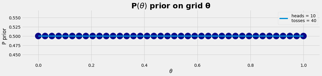
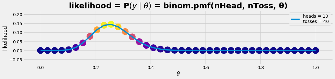
For the application the following vectors are used:

nθ = 40    # resolution: number of θ-points
nToss = 40 # experiment: tossing nToss times
nHead = 10 # result:  heads out of nToss
df = get_posterior(nθ , nHead, nToss); #df

Python code

import numpy as np
import pandas as pd
from scipy import stats
from matplotlib import pyplot as plt
import matplotlib.colors as mclr

def plot_gr00(X,Y,xLabel,yLabel,nHead,nToss,θ,xv,vlabel,grTitel):
    with plt.style.context('fivethirtyeight'):         
         fig = plt.figure(figsize=(35,3)) ;       
         ax1 = fig.add_subplot(121);
         a1size = np.ones_like(X)*500;        
         ax1.scatter(X, Y, marker='o', s=a1size,  c=Y, edgecolors='w',cmap="plasma");
         ax1.plot(X,Y, label='y = {}\n n = {} \n θ = {} '.format(nHead, nToss, θ));
         ax1.vlines(xv, 0, 0.2, linestyle='--',colors='r', lw=5,label=vlabel)
         plt.legend(loc=0)       
         plt.xlabel(xLabel);  plt.ylabel(yLabel);
         plt.title(grTitel, fontsize=25, fontweight='bold');
         plt.show()

def plot_gr01(X,Y,xLabel,yLabel,grTitel):
    with plt.style.context('fivethirtyeight'):         
         fig = plt.figure(figsize=(35,3)) ;       
         ax1 = fig.add_subplot(121);
         a1size = np.ones_like(X)*500;        
         ax1.scatter(X, Y, marker='o', s=a1size,  c=Y, edgecolors='w',cmap="plasma");
         ax1.plot(X,Y, label='heads = {}\ntosses = {}'.format(nHead, nToss));
         plt.legend(loc=0)       
         plt.xlabel(xLabel);  plt.ylabel(yLabel);
         plt.title(grTitel, fontsize=25, fontweight='bold');
         plt.show()

def get_likelihood(θ,n):
    ay = np.arange(n)
    p_lklhd= stats.binom.pmf(ay,n,θ)    
    plot_gr00(ay, p_lklhd, r'$y$','P','$heads$',n,θ,
              θ*nToss,'$P_{max}(y = n \cdot θ)$',
              '$P(y\mid θ_{fix}) = binom.pmf(y, n, θ_{fix})$')   
    aθ = np.linspace(0, 1, n)
    y  = 10
    p_lklhd= stats.binom.pmf(y,n,aθ)
    plot_gr00(aθ, p_lklhd, r'$θ$','P','$10$',n,'bias',
              y/n,'$P_{max}(θ = y/n)$',
              '$P(y_{fix}\mid θ) = binom.pmf(y_{fix}, n, θ)$') 

def get_pTable(n):
    Y = np.arange(n)
    θ = np.linspace(0, 1, n)
    A = np.zeros((n,n))
    for y in Y:
        A[y,:] = stats.binom.pmf(y,n-1,θ) 
    ax = np.outer(Y,np.ones_like(θ))  # X = ix.T * ones(iy)
    ay = np.outer(np.ones_like(Y),θ)  # Y = ones(ix) * iy.T
    with plt.style.context('fivethirtyeight'):      
        fig = plt.figure(figsize=(7,7)) 
        ax1 = fig.add_subplot(111)
        ax1.scatter(ax, ay, s= 5+150*A**(1/10), c=A**(1/9), edgecolors='w',cmap="plasma")
        plt.xlabel('y');  plt.ylabel('θ');
        plt.title('p = binom.pmf(y, n, θ)', fontsize=15, fontweight='bold');
    plt.show()

def get_posterior(nθ, nHead, nToss):
    θ      = np.linspace(0, 1, nθ)
    p_prio = np.repeat(0.5, nθ)
    p_lklhd= stats.binom.pmf(nHead, nToss, θ)
    p_post = p_lklhd * p_prio / sum(p_lklhd * p_prio)
    plot_gr01(θ, p_prio,r'$\theta$','P prior','P$( θ )$ prior on grid θ')
    plot_gr01(θ, p_lklhd,r'$\theta$','likelihood','likelihood = P$(y \mid θ )$ = binom.pmf(nHead, nToss, θ)')
    plot_gr01(θ, p_post,r'$\theta$','P posterior','P$(θ \mid y)$ posterior')    
    df = pd.DataFrame({'θ': θ, 'p_prio':p_prio, 'p_lklhd': p_lklhd,'p_post':p_post}) 
    return df