Computational Fluid Dynamics: An explict Python Schema for the 2dim Diffusion Equation

Stationary equation

The stationary diffusion equation with constant diffusion coefficients is given in coordinate free representaion as

$$ \begin{eqnarray} - K \cdot\nabla^2 u &=& S_{diff} \end{eqnarray} $$

Using cartesian coordinates we can write

$$ \begin{eqnarray} - K^x \frac {\partial^2 u}{\partial{x}^2} - K^y \frac {\partial^2 u}{\partial{y}^2} &=& S_{diff}\\ - K^x u_{xx} - K^y u_{yy} &=& S_{diff} \end{eqnarray} $$

Time dependent equation

The time dependent diffusion equation is given as

$$ \begin{eqnarray} \frac {\partial u}{\partial{t}}- K \cdot\nabla^2 u &=& S_{diff} \\ u_t - K^x u_{xx} - K^y u_{yy} &=& S_{diff} \end{eqnarray} $$

Explicit finite difference (FD) discretization with equidistant cartesian grid

Time dependent solution

$$ \frac{u_{i,j}^{n+1} - u_{i,j}^{n}}{\Delta t} -K^x \frac{u_{i+1,j}^{n} - 2u_{i,j}^{n} + u_{i-1,j}^{n}}{(\Delta x)^2} -K^y \frac{u_{i,j+1}^{n} - 2u_{i,j}^{n} + u_{i,j-1}^{n}}{(\Delta y)^2} = S^{diff}_{i,j} $$

$$ u_{i,j}^{n+1} = u_{i,j}^{n} + \Delta t \bigg( K^x \frac{u_{i+1,j}^{n} - 2u_{i,j}^{n} + u_{i-1,j}^{n}}{(\Delta x)^2} +K^y \frac{u_{i,j+1}^{n} - 2u_{i,j}^{n} + u_{i,j-1}^{n}}{(\Delta y)^2} + S^{diff}_{i,j} \bigg) $$

$$ u_{i,j}^{n+1} = u_{i,j}^{n} + \Delta t \cdot d u^n $$

The numerical solution can be found by propagating $u$ from one timpstep $n$ to the next timesptep $n+1$

Stationary solution

$$ -\frac{K^x }{(\Delta x)^2} \bigg(u_{i+1,j}^{n+1} - 2u_{i,j}^{n+1} + u_{i-1,j}^{n+1} \bigg) -\frac{K^y }{(\Delta y)^2} \bigg(u_{i,j+1}^{n+1} - 2u_{i,j}^{n+1} + u_{i,j-1}^{n+1} \bigg) = S^{diff}_{i,j} $$

Using compass notation we can write

$$ A^E \cdot u_{i+1,j}^{n+1} + A^W \cdot u_{i-1,j}^{n+1} + A^N \cdot u_{i,j+1}^{n+1} + A^S \cdot u_{i,j-1}^{n+1} - A^P \cdot u_{i,j}^{n+1} = RHS_{diff} $$

with

$$ \begin{eqnarray} A^E &=& -\frac{K^x }{(\Delta x)^2} \\ A^W &=& -\frac{K^x }{(\Delta x)^2} \\ A^N &=& -\frac{K^y }{(\Delta y)^2} \\ A^S &=& -\frac{K^y }{(\Delta y)^2} \\ A^P &=& A^E + A^W + A^N + A^S\\ RHS_{diff} &=& S^{diff}_{i,j} \end{eqnarray} $$

To find a solution the following equation system for the unknown $u$ at all grid points has to be solved simultaneously:

$$ \begin{eqnarray} \mathbf{A \cdot u} &=& \mathbf{RHS} \end{eqnarray} $$

We will adress that in a seperate post.

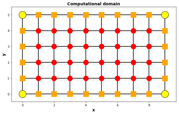
Boundary condtions (BC) for the explicit schema

When using the explicit schema only the interior (red) points of the grid are evaluated usually. So the (orange) points at the boundary can be used to store fiexed values, or they can be upgraded at each time step in such a way that some flux boundary conditions are fullfilled.

ComputationalDomain()

png

Fixed values at the boundary (Dirichlet BC)

Let's assume we want a fixed value $uBC$ at the east boundary. So we just store this value in u[nx,iy]:

$$ u[nx,iy] = uBC $$

Prescribed flux at the boundary (Neuman BC)

Let's assume we want a prescribed flux $F^e$ at the east boundary. We use the discretized form of the flux and solve it so that we can update u[nx,iy] at each iteration:

$$ \begin{eqnarray} K^x\frac{\partial {u} }{\partial {x}} &=&K^x\frac{u[nx,iy] - u[nx-1,iy]}{\Delta x} &=& F^e \\ u[nx,iy] &=& u[nx-1,iy] + \frac{F^e\Delta x}{K^x} \end{eqnarray} $$

For the most often used flux $F^e = 0$ the update becomes

$$u[nx,iy] = u[nx-1,iy]$$

An example

Equation: $\frac {\partial u}{\partial{t}}- K \cdot\nabla^2 u = S_{diff}$
Domain: $D = [-1 \enspace x \enspace 1]^2$
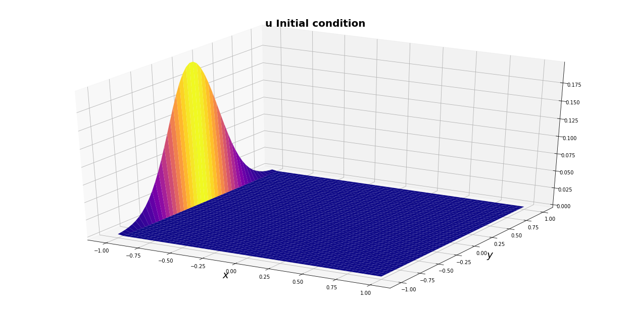
fix BC at west boundary: $u = 0.2*exp(-20\cdot y^2)$, where y is the y-coordinate of D
fix BC at north and south boundary: $u = 0$
grad BC at east boundary: $u_x = 0$
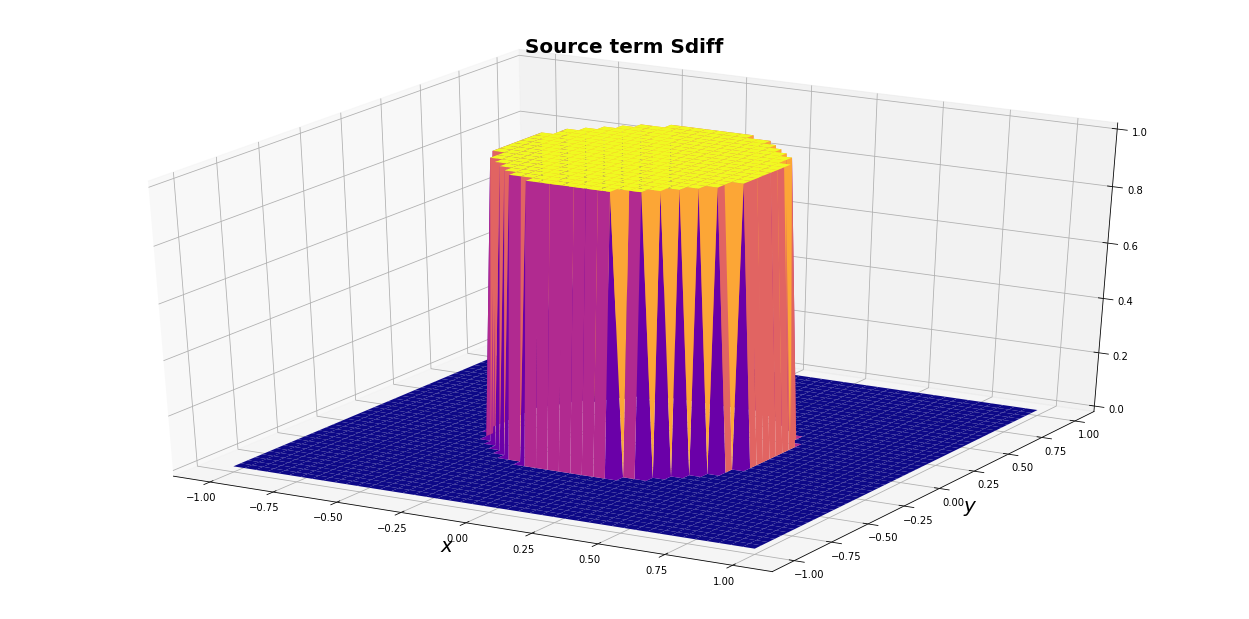
Source : $S = round(1-R)$ with $R = \sqrt{(x^2 + y^2)}$
Diffusivities: $K^x = K^y = 1$
Interior initial condition: $u=0$
Discretization: Finite Differences (FD) on an equidistant cartesian grid
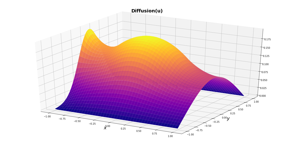
since the boundary conditions do not change, the solution converges to a stationary state

import numpy as np
import matplotlib.pyplot as plt
import matplotlib.colors as mclr
from matplotlib import cm
from mpl_toolkits.mplot3d import Axes3D ##library for 3d projection plots
from IPython.core.pylabtools import figsize

np.set_printoptions(formatter={'float': '{: 0.3f}'.format})

def grafics(Z,titel):
    fig = plt.figure(figsize=(22,11))
    ax = fig.add_subplot(111)
    ax = fig.gca(projection='3d')
    ax.plot_surface(x, y, Z, rstride=1, cstride=1, cmap=cm.plasma,
            linewidth=0, antialiased=True)
    ax.set_xlabel('$x$',fontsize=20,fontweight='bold')
    ax.set_ylabel('$y$',fontsize=20,fontweight='bold');
    plt.title(titel, fontsize=20,fontweight='bold')
    plt.show()

Python code for the 2dimensional explicit time dependent diffusion equation

#---- input section ----------------------------
nx = 46; ny = 46;         # number of grig points
Lx =  2; Ly =  2;         # lenght of domain
nt = 9000                 # number of iterations
dt = 0.0001               # time step
Kx = 1.0; Ky = 1.0;       # diffusivities

#---- evaluate input ---------------------------
dx = Lx/(nx-1); dx2 = dx*dx
dy = Ly/(ny-1); dy2 = dy*dy

#---- generate grid for grafics ----------------
ix = np.linspace(0, 1 ,nx)-0.5
iy = np.linspace(0, 1, ny)-0.5
x  = Lx * np.outer(ix,np.ones_like(iy))  
y  = Ly * np.outer(np.ones_like(ix),iy)  

def set_InitialValue():
    u = np.zeros((nx, ny))
    Sdiff = np.zeros((nx, ny)); R = np.sqrt(x*x + y*y)
    Sdiff = np.round(1.0 - R)
    return u, Sdiff

def set_FixBC(u):
    #--- west boundary ---
    jx = 0; jy = slice(0,ny);  u[jx,jy] = 0.2*np.exp(-20*iy[jy]**2)
    return u

def set_GradBC(u):
    #--- east boundary ---
    jx = nx-1; jxm = jx-1; jy = slice(0,ny);  u[jx,jy] = u[jxm,jy]
    return u

def du(u,Sdiff):
    jx = slice(1,nx-1); jxm = slice(0,nx-2); jxp = slice(2,nx)
    jy = slice(1,ny-1); jym = slice(0,ny-2); jyp = slice(2,ny)
    DU = np.zeros_like(u)
    DU[jx,jy] = (u[jxp,jy] - 2.0*u[jx,jy] + u[jxm,jy])*Kx/dx2 + \
                (u[jx,jyp] - 2.0*u[jx,jy] + u[jx,jym])*Ky/dy2 + \
                Sdiff[jx,jy]
    return DU

#------- initialize -------------------------
u, Sdiff = set_InitialValue()
u = set_FixBC(u)

#---- graphical display --------------
grafics(u, "u Initial condition")

#------- iterate -------------------------
for n in range(nt + 1):
    u = set_GradBC(u)
    un = u + dt*du(u,Sdiff)
    u = un.copy()

png

#---- graphical display --------------
grafics(Sdiff, "Source term Sdiff")

png

#---- graphical display --------------
grafics(u,"Diffusion(u)")

png

Grafics for the computational domain

def ComputationalDomain():

    nx = 10; ny = 6

    #---- set the 1-dimensional index arrays in x- and y-direction
    ix = np.linspace(0,nx-1,nx, dtype=int)
    iy = np.linspace(0,ny-1,ny, dtype=int)

    #---- define the grid using the outer product -----------
    x = np.outer(ix,np.ones_like(iy))  # X = ix.T * ones(iy)
    y = np.outer(np.ones_like(ix),iy)  # Y = ones(ix) * iy.T

    ss = 1
    figsize(ss*nx,ss*ny)
    area = 150

    myCmap = mclr.ListedColormap(['white','white'])
    plt.axes().pcolormesh(x, y, np.zeros_like(x), edgecolors='k', lw=1, cmap=myCmap)

    #--- sw corner ----------------------
    jx = 0;  jxp = 1;
    jy = 0;  jyp = 1;
    xp = x[jx,jy ];   yp = y[jx,jy ];  
    plt.scatter(xp,yp, s=4*area, c='yellow',edgecolors='k')

    #--- se corner ----------------------
    jx = nx-1; jxm = nx-2; 
    jy = 0;    jyp = 1;
    xp = x[jx,jy ];   yp = y[jx,jy ]; 
    plt.scatter(xp,yp, s=4*area, c='yellow',edgecolors='k')

    #--- nw corner ----------------------
    jx = 0;     jxp = 1; 
    jy = ny-1;  jym = ny-2;
    xp = x[jx,jy ];   yp = y[jx,jy ]; 
    plt.scatter(xp,yp, s=4*area, c='yellow',edgecolors='k')

    #--- ne corner ----------------------
    jx = nx-1;  jxm = nx-2; 
    jy = ny-1;  jym = ny-2;
    xp = x[jx,jy ];   yp = y[jx,jy ]; 
    plt.scatter(xp,yp, s=4*area, c='yellow',edgecolors='k')

    #--- south boundary -----------------------------
    jx = slice(1,nx-1);  jxm = slice(0,nx-2);  jxp = slice(2,nx);  
    jy = 0; jyp = 1
    xp = x[jx,jy ];   yp = y[jx,jy ];
    plt.scatter(xp,yp, s=2*area, c='orange',marker='s')

    #--- north boundary -----------------------------
    jx = slice(1,nx-1); jxm = slice(0,nx-2);  jxp = slice(2,nx);  
    jy = ny-1; jym = ny-2
    xp = x[jx,jy ];   yp = y[jx,jy ];  
    plt.scatter(xp,yp, s=2*area, c='orange',marker='s')

    #--- west boundary -----------------------------
    jx = 0;   jxp = 1;  
    jy = slice(1,ny-1);  jym = slice(0,ny-2);  jyp = slice(2,ny); 
    xp = x[jx,jy ];   yp = y[jx,jy ]; 
    plt.scatter(xp,yp, s=2*area, c='orange',marker='s')

    #--- east boundary -----------------------------
    jx = nx-1;   jxm = nx-2;  
    jy = slice(1,ny-1);  jym = slice(0,ny-2);  jyp = slice(2,ny); 
    xp = x[jx,jy ];   yp = y[jx,jy ];
    plt.scatter(xp,yp, s=2*area, c='orange',marker='s')

    #--- interior area ---------------------------------
    jx = slice(1,nx-1); jxm = slice(0,nx-2); jxp = slice(2,nx)
    jy = slice(1,ny-1); jym = slice(0,ny-2); jyp = slice(2,ny)
    xp = x[jx,jy ];   yp = y[jx,jy ]; 
    plt.scatter(xp,yp, s=2*area, c='red')

    plt.xlabel('x',fontsize=14, fontweight='bold')
    plt.ylabel('y',fontsize=14, fontweight='bold')
    plt.title('Computational domain',fontsize=14, fontweight='bold')
    plt.axes().set_aspect('equal')
    #plt.axes().set_facecolor("black")
    plt.show()