MetaAnalysis 02: A Medical Decision Tree Intro

Decision tree for state of health

We denote different states of health, e.g., healthy, ill, dead, with $H^h, H^i, H^d$. We can assume that $H^i$ can be any health state bewteen $H^h$ and $H^d$. But this choice is not mandatory. We can choose any state of health $H^A, H^B, H^C$.

Let's assume an individual has at time $t_o$ a health state $i$, which is denoted as $H_0^i$. The individual may be confronted with the choice between $H_0^i$ and the uncertain prospect $[H_1^h, H_1^d]^T$ or $[H_1^h, H_1^i, H_1^d]^T$ due to a therapy. $p$, $q$, and $(1-p-q)$ are the probablities for the different outcomes. A decision tree is concerned with the problem of changing the state of health from $\mathbf{H}_0$ to $\mathbf{H}_1$ including the uncertainities of the different outcomes.

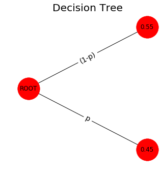
The 2-states model of a therapy

A simpler model may comprise two states of health as prospect of a therapy $T$

$$ \begin{equation} \begin{array}{rcl} H_0^i & \xrightarrow[]{T} & \left[\begin{matrix} H^h_1\\ H^d_1\end{matrix}\right] \\ \end{array} \end{equation} $$

By summarizing the probablilties of the different outcomes as

$$ \begin{equation} \begin{array}{rcl} \mathbf{p} & = & \left[\begin{matrix}p & (1-p)\end{matrix}\right] & = & diag(\mathbf{P}) \end{array} \end{equation} $$

we can form the operator as matrix $\mathbf{P}$

$$ \begin{equation} \begin{array}{rcl} \mathbf{P}& = & \left[\begin{matrix}p & 0\\ 0 & (1-p) \end{matrix}\right] \end{array} \end{equation} $$

and we can now write the decision tree as a Markov chain model with one time step as

$$ \begin{equation} \begin{array}{rcl} H_0^i & \xrightarrow[]{T} & \mathbf{P}\cdot\mathbf{H}_1 \\ & & = \left[\begin{matrix}p \cdot H^h_1\\ (1-p) \cdot H^d_1\end{matrix}\right] \end{array} \end{equation} $$

With \(\mathbf{p} = \left[

\begin{matrix}p & (1-p)\end{matrix}

\right] = \left[

\begin{matrix}0.45 & 0.55\end{matrix}

\right]\) this model has this tree:

tree_2()

png

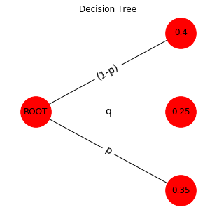
The 3-states model

$$ \begin{equation} \begin{array}{rcl} H_0^i & \xrightarrow[]{T} & \mathbf{H}_1 = \left[\begin{matrix}H^h_1 \\ H^i_1 \\H^d_1\end{matrix}\right] \\ & \textrm{with} & \mathbf{p} = \left[\begin{matrix}p & q & (1-p-q)\end{matrix}\right] & = & diag(\mathbf{P})\\ & \textrm{and} & \mathbf{P} = \left[\begin{matrix}p & 0 & 0 \\ 0 & q & 0 \\ 0 & 0 & (1-p-q)\end{matrix}\right] \\ \end{array} \end{equation} $$

The decison tree as a Markov chain model with one time step is

$$ \begin{equation} \begin{array}{rcl} H_0^i & \xrightarrow[]{T} & \mathbf{P}\cdot\mathbf{H}_1 \\ & & = \left[\begin{matrix}p \cdot H^h_1\\ q \cdot H^i_1 \\(1-p-q) \cdot H^d_1\end{matrix}\right] \end{array} \end{equation} $$

With

$$\mathbf{p} = \left[\begin{matrix}p & q &(1-p-q)\end{matrix}\right] = \left[\begin{matrix}0.35 & 0.25 & 0.40\end{matrix}\right]$$

this model has this tree:

tree_3()

png

A 2-level model of a compounded therapy or diagnosis

If a diagnostic test and/or a therapeutical intervention is compounded by two distinguishable steps the model becomes:

$$ \begin{equation} \begin{array}{rcl} H_0^i & \xrightarrow[]{T_1} & \mathbf{P}\cdot\mathbf{H}_1 & \xrightarrow[]{T_2} &\mathbf{R} \cdot (\mathbf{P}\cdot\mathbf{H}_1) \end{array} \end{equation} $$

With

$$ \begin{equation} \begin{array}{rcl} \mathbf{p} & = & \left[\begin{matrix}p & q &(1-p-q)\end{matrix}\right] & = & \left[\begin{matrix}0.35 & 0.25 & 0.40\end{matrix}\right] \\ \mathbf{r} & = & \left[\begin{matrix}r & (1-r)\end{matrix}\right] & = & \left[\begin{matrix}0.10 & 0.90\end{matrix}\right] \end{array} \end{equation} $$

The decision tree has now the following form:

tree_23()

png

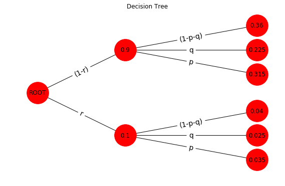
Evaluation of the tree

On right side of the tree are 6 end points, called foils. A branche is the connection between a foil and the root. On each of this 6 branches the probabilities of p and r are multiplied. In order to evaluate all probablities of the foils one can imagine that p and r build a grid that can be computed by the outer product as demonstrated here and here in a different context.

The matrix $\mathbf{\Pi}$ with the probabilities of the foils can be computed by

$$ \begin{equation} \begin{array}{rcl} \mathbf{\Pi} & = & \mathbf{r}^T \cdot\mathbf{p} & = &\left[\begin{matrix}r \\ (1-r)\end{matrix}\right] \cdot \left[\begin{matrix}p & q &(1-p-q)\end{matrix}\right]\\ & & & = & \left[\begin{matrix}p r & q r & (1-p-q) r\\(1-r) p & (1-r) q & (1-p-q) (1-r)\end{matrix}\right] \end{array} \end{equation} $$

Analytically this can be shown with SymPy, a Python library for symbolic mathematic

import sympy as s
s.init_printing()
from IPython.display import display

p1,r1 = s.symbols("(1-p-q) (1-r)")

p = s.Matrix([['p','q', p1]])
r = s.Matrix([['r', r1]])
T = r.T*p   #outer product

#display(p); display(r); 
display(T)

$$\left[\begin{matrix}p r & q r & (1-p-q) r\\(1-r) p & (1-r) q & (1-p-q) (1-r)\end{matrix}\right]$$

Numerically this can be shown with the numpy function np.outer

#--- input --------
p = 0.35;  q = 0.25;   pn = np.array([ p, q,  1-p-q])
r = 0.10;              rn = np.array([ r, 1-r]      )
#--- outer product --------
Π  = np.outer(rn, pn)
print('Π =') ; print(Π)

Π =
[[ 0.035  0.025  0.04 ]
 [ 0.315  0.225  0.36 ]]

All branches of the decision tree that connect the root with the foils are evaluatetd now.

The Python code

import numpy as np
import networkx as nx
import matplotlib.pyplot as plt

def treeGrafics(G,figX,figY):
    from IPython.core.pylabtools import figsize

    with plt.style.context('fivethirtyeight'): 
        fig = plt.figure(figsize=(figX,figY))
        axes1 = fig.add_subplot(1, 1, 1)
        pos=nx.get_node_attributes(G,'pos')
        plt.title('Decision Tree')
        nx.draw(G, pos, with_labels=True, arrows=False, node_size=1900)
        edge_labels =dict([((u, v), d['label']) 
                   for u, v, d in G.edges(data=True)])
        nx.draw_networkx_edge_labels(G, pos, edge_labels=edge_labels,font_size=14)
        plt.axis('off')
        plt.show()

def setTriage_00(G,nodeIn,pn,ps,dx,dy,f,):
    pos=nx.get_node_attributes(G,'pos')
    pL = len(pn)
    for i,pj in enumerate(pn):
        ii = f*2*(i/(pL-1)-0.5) + dy
        G.add_node(pj, pos=(pos[nodeIn][0]+dx, pos[nodeIn][1]+dy + ii))
        G.add_edge(nodeIn, pj, label=ps[i])
    return G

def setTriage_11(G,nodeIn,pn,ps,dx,dy,f):
    pos=nx.get_node_attributes(G,'pos')
    pL = len(pn)
    for i,pj in enumerate(pn):
        ii = f*2*(i/(pL-1)-0.5) + dy
        G.add_node(pj*nodeIn, pos=(pos[nodeIn][0]+dx, pos[nodeIn][1]+dy + ii))
        G.add_edge(nodeIn, pj*nodeIn, label=ps[i])
    return G

def tree_2():
    #--- input --------
    p = 0.45;
    figX = 4.5;  figY = 5

    #--- compute tree ----------
    pn = np.array([ p,    1-p]  )
    ps = np.array(['p', '(1-p)'])

    with plt.style.context('fivethirtyeight'): 
        G=nx.DiGraph()
        G.add_node("ROOT", pos=(0, 0))
        pos=nx.get_node_attributes(G,'pos')
        G = setTriage_00(G,"ROOT", pn,ps, 2, 0, 3.5)
        treeGrafics(G,figX,figY)

def tree_3():
    #--- input --------
    p = 0.35; q = 0.25
    figX = 4.5;  figY = 5

    #--- compute tree ----------
    pn = np.array([ p,  q,  1-p-q]  )
    ps = np.array(['p','q','(1-p)'])

    G=nx.DiGraph()
    G.add_node("ROOT", pos=(0, 0))
    pos=nx.get_node_attributes(G,'pos')
    G = setTriage_00(G,"ROOT", pn,ps, 2, 0, 3.5)
    treeGrafics(G,figX,figY)

def tree_23():
    #--- input --------
    p = 0.35; q = 0.25
    r = 0.10
    figX = 9.5;  figY = 6 

    #--- compute tree ----------    
    pn = np.array([ p,  q,   1-p-q]  )
    ps = np.array(['p','q','(1-p-q)'])

    rn = np.array([ r,   1-r]  )
    rs = np.array(['r','(1-r)'])

    G=nx.DiGraph()
    G.add_node("ROOT", pos=(0, 0))

    pos=nx.get_node_attributes(G,'pos')
    G = setTriage_00(G,"ROOT", rn,rs, 2, 0, 3.5)

    for rni in rn:
        G = setTriage_11(G,rni,pn,ps, 3, 0.0, 2.0) 

    treeGrafics(G,figX,figY)