Computational Fluid Dynamics 02: Body-fitted grids without for loops

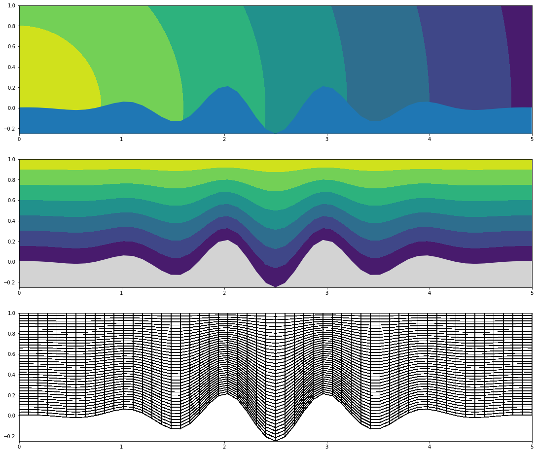
Python code for a terrain-following grid

In this example the terrain-followin property is executed in the y-direction. The x-coordinate is determined as in the rectangular case in the previous example. At each x-grid point the y-coordinate is computed as

$$ y = y_{bottom} + \eta \cdot (y_{top} - y_{bottom}) = y_{bottom} + \eta \cdot dY $$

where $\eta$ varies between 0..1. In the following code iy has the role of $\eta$ . Again the outer product completes the grid efficiently.

def scale01(z):   #--- transform z to [0 ..1]
    return (z-np.min(z))/(np.max(z)-np.min(z))

def scale11(z):   #--- transform z to [-1 ..1]
    return 2.0*(scale01(z)-0.5)

import numpy as np

nx = 55; ny = 39
Lx = 5.0;  Ly = 1.0
ix = np.linspace(0,nx-1,nx)/(nx-1)
iy = np.linspace(0,ny-1,ny)/(ny-1)

#--- set some fancy south boundary ----
A = 0.5; B = 1.0; C = 5.0; D = 0.25
south_boundary = B*np.exp(-(scale11(ix)/A)**2) * D*np.cos(scale01(ix)*C*2.0*np.pi)
north_boundary = np.ones_like(south_boundary)
dY =  north_boundary - south_boundary

#--- use the outer product to complete the 2D x-/y-coord
x = np.outer(ix,np.ones_like(iy))
y = np.outer(dY,iy) + np.outer(south_boundary,np.ones_like(iy))

The graphical display

import matplotlib.pyplot as plt
import matplotlib.colors as mclr
#---- grafics ------------------------------------------------
#--- scale for the graphics ---------------
X=x*Lx;  Y=y*Ly

#--- set some fancy Z-values ---------
Z1 = np.sqrt(X*X + Y*Y)
Z2 = np.outer(np.ones_like(dY),iy)
Z3 = Y

#---- experiment with the graphics --------
fig = plt.figure(figsize=(22,22)) 
ax1 = fig.add_subplot(411)
ax1.contourf(X, Y, -Z1)
ax1.fill_between(ix*Lx, south_boundary*Ly, min(south_boundary)*Ly)
ax1.set_aspect('equal')

ax1 = fig.add_subplot(412)
ax1.contourf(X, Y, Z2)
#ax1.pcolormesh(X, Y, Z2, edgecolors='w',cmap="plasma")
ax1.fill_between(ix*Lx, south_boundary*Ly, min(south_boundary)*Ly,facecolor='lightgrey')
ax1.set_aspect('equal')

myCmap = mclr.ListedColormap(['white','white'])
ax4 = fig.add_subplot(413)
ax4.pcolormesh(X, Y, np.zeros_like(X), edgecolors='k', lw=0.75, cmap=myCmap)
ax4.set_aspect('equal')
plt.show()

png

$$ $$

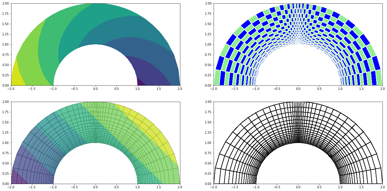
Python code for a terrain-following polar grid

ix has the role of the angle $\phi$
ix is transformed to sx so that the grid points will be concentrated in the middle of the $\phi$-domain
iy has the role of the radius $r$
iy is transformed to sy so that the grid points will be concentrated at the lower boundary of the $r$-domain
(x,y) is the grid in polar coordinates ($\phi, r$)
(x,y) is transformed to the cartesian coordinates (X,Y)

import numpy as np
import matplotlib.pyplot as plt
import matplotlib.colors as mclr

nx = 38; ny = 18
ix = np.linspace(0,nx-1,nx)/(nx-1)
iy = np.linspace(0,ny-1,ny)/(ny-1)

#---- stretching in x- = angular-direction ---------
ixx =  np.linspace(0,nx-2,nx-1)/(nx-2)
dxmin = 0.1;                                # minimal distance as control parameter
dxx = 1.0-np.sin(ixx*np.pi) + dxmin         # model the distances
sx = np.array([0])                          # set the starting point
sx = scale01(np.cumsum(np.append(sx,dxx)))  # append the distances and sum up

#---- stretching in y- = radial-direction ---------
yStretch = 0.5; yOffset = 2.95                    # control parameters
sy = scale01(np.exp((yStretch*(yOffset+iy))**2)); # exp-stretching

#---- complete as polar coordinates --------------
tx = np.pi * sx            # use ix as angel phi
ty =   1.0 + sy            # use iy as radius r [1.0 .. 2.0]

x = np.outer(tx,np.ones_like(ty))  
y = np.outer(np.ones_like(tx),ty)  

#---- transform to cartesian coordinates ---------
X = y * np.cos(x) # transform to cartesian x-coord
Y = y * np.sin(x) # transform to cartesian y-coord

The graphical display

#---- grafics---------------------------------------------
fig = plt.figure(figsize=(22,11)) 
ax1 = fig.add_subplot(221)
ax1.contourf(X, Y, x + y)

ax2 = fig.add_subplot(222)
c1, c2 = np.meshgrid(iy*(ny-1),ix*(nx-1))
myCmap = mclr.ListedColormap(['blue','lightgreen'])
ax2.pcolormesh(X, Y, (-1)**(c1+c2), edgecolors='w', lw=0.75, cmap=myCmap)

myCmap = mclr.ListedColormap(['white','white'])
ax3 = fig.add_subplot(223)
ax3.pcolormesh(X, Y, np.zeros_like(X), edgecolors='k', lw=0.5, cmap=myCmap, alpha=0.5)
ax3.contourf(X, Y, X+Y, alpha=0.75)

ax4 = fig.add_subplot(224)
ax4.pcolormesh(X, Y, np.zeros_like(X), edgecolors='k', lw=1, cmap=myCmap)
plt.show()

png