
- Sa 19 Mai 2018
- MetaAnalysis
- Peter Schuhmacher
- #numerical, #statistics, #python, #bayesian
The Task
We want to have a number of samples that follow a certain distribution, which means that we want to have at the end more samples in the region where the density of the PDF (probability density function) is high and less samples in the regions with lower density.
In the following example our samples \(\mathbf{x}\) will just be the geometrical (x,y)-coordinates in the plane. In an application however a sample \(\mathbf{x}\) might be a multidimensional vector assembling some features as e.g.
What does the Metropolis sampler ?
In the 2-dimensional case the sampler returns a list with the (x,y)-coordinates of the samples. As an imput it uses an arbitrary PDF. In a previous example we have built a CDF (cumulative distribution function) first. But the Metropolis sampler uses the PDF without building a CDF.
There are many different Markov Chain Monte Carlo-type samplers. Historically Metropolis was the first, Metropolis-Hastings a later improvement, Gibbs sampler and more.
What does the Markov Chain part ?
The MCMC sampler searches the samples systematically. Given a sampling point then the MCMC sampler moves to the next sampling point if this represents a higher probability. This asserts a walk in direction of the region with high probability densitiy.
So beeing at a certain sampling point, the transition probability to the next sampling point is given. That's the Markov aspect of the walk. Note that a Markov matrix with the transition probabilities is not built explicitly. The algorithm applies the principle locally and so the result is a Markov chain, which means a chain of \(\mathbf{x}\)-positions.
What is the Monte Carlo random noise good for ?
A pure Markov walk faces a series of problems.
- imagine the PDF to be a mountain with a distinctive peak. How to continue the walk when the order is strictely: "Move to the top!" ?
- imagine the PDF to be two islands in a flat sea of zeros. In which direction is the walk to be continued in a slope-less zero-plane ?
- imagine you choose randomly a starting point and follow the continuos and monotonic Markov path. What would be the path from a different starting point a little bit apart ?
Of course each of these points is adressed by theory stating that the Markov part should be somehow well-behaved, e.g. :
- The imaginary Markov matrix must not lead to an oscillatory behaviour of the chain.
- The imaginary Markov matrix should be fully occupied in an order that each point of the space can be reached.
The Monte Carlo part helps to circumvent the faced problems. The Markov Chain part should give a usefull tendency but not too strictely. So Markov Chain and Monte Carlo are something like Ying and Yang.
The cases
With the Metropolis-Hasting algorithm we sample first and reconstruct then the following two examples of 2-dimensional PDF :
#--- create the grid ---------------------------
mx = 70; Dx = 11; xm = np.linspace(-Dx,Dx,mx)
my = mx; Dy = 11; ym = np.linspace(-Dy,Dy,my)
Xm = np.outer(xm,np.ones_like(ym))
Ym = np.outer(np.ones_like(xm),ym)
#--- plot the cases -----------------------------
case=1; rv1,rv2 = q_setup(case); rvPDF1 = q(Xm,Ym)
case=2; rv1,rv2 = q_setup(case); rvPDF2 = q(Xm,Ym)
plot_grafics_X(Xm,Ym,rvPDF1,rvPDF2,8)
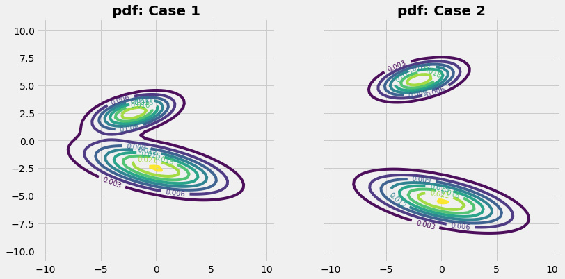
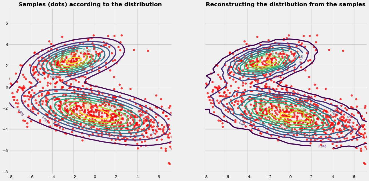
Case 1
The given PDF (isolines) seems to cover a connected area. The graphics on the left side shows the samples (red dots) chosen by the Mtreopolis-Hasting algorithm. For easier visual interpretation the run contains only a few number of samples (~\(10^4\)). By visual inspection we can see that the samples cover fairly the regions of the PDF.
The graphics on the right side shows the reconstruction of the PDF (isolines) based on the samples. For the reconstruction with prepare a grid of control volumes. A control volumne acts as a counter: Each time when a sample is in the control volume it counts this event. This gives the distribution of the frequency. To get a reliable reconstruction of the PDF the run needs a large number of samples (~\(10^6\)).
#===== run case 1 =========================
#----- setup the target distribution ------
case = 1; rv1,rv2 = q_setup(case)

#----- run the sampling with Metropolis-Hastings ------
N = 12000; s = 10;  case=1;  Ns = N/s
samples = np.array(MetropolisHastings(N,s))

#---- reconstruct the distribution from the samples
Xc,Yc,Zdistr,counts,sam1 = reconstruct(samples)
plot_grafics(Xc,Yc,Zdistr,counts,sam1)
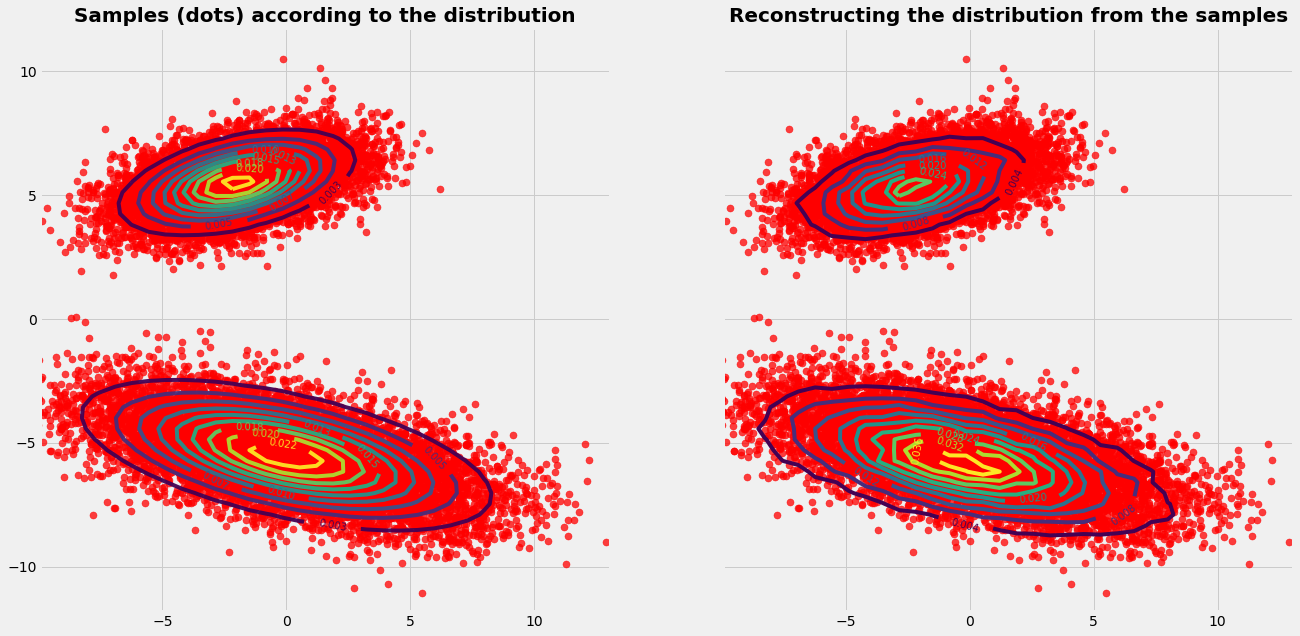
Case 2
In case 2 the regions of the different parts of the probability distribution are hardly connected. We have now the situation with two probability islands in the sea of zeros. The theoretical requirement, that the Markov Chain must be able to reach any point, is not fullfilled (because of too many zeros in the imaginary Markov matrix).
When experimenting with the sampling procedure we realize that we need now more samples (~\(10^5\)) than in case 1. Otherwise only one part (one island) of the PDF might be sampeld.
Despite unfavorable and rule breaking conditions, the algorithm is able to sample both important areas of the PDF. This is due to the power of the Monte Carlo part.
#===== run case 2 =========================
#----- setup the target distribution ------
case = 2; rv1,rv2 = q_setup(case)

#----- run the sampling with Metropolis-Hastings ------
N = 200000; s = 10;  case=1;  Ns = N/s
samples = np.array(MetropolisHastings(N,s))
#---- reconstruct the distribution from the samples
Xc,Yc,Zdistr,counts,sam1 = reconstruct(samples)
plot_grafics(Xc,Yc,Zdistr,counts,sam1)
The sampling algorithm
import numpy as np
import pandas as pd
from scipy.stats import multivariate_normal
import matplotlib.cm as cm
import matplotlib.mlab as mlab
import matplotlib.pyplot as plt
def AR(w): return w*np.ones((1,1)) # a little hack to transform a float into a (1,1)-matrix

def q_setup(case):                 # prepare the PDF as input parameter
    if case == 1:
        muXa=-2; muYa= 2.5; varXXa= 5; varYYa=1; varXYa= 0; varYXa= 1
        muXb= 0; muYb=-2.5; varXXb=15; varYYb=2; varXYb=-0; varYXb=-3
    if case == 2:
        muXa=-2; muYa= 5.5; varXXa= 5; varYYa=1; varXYa= 0; varYXa= 1
        muXb= 0; muYb=-5.5; varXXb=15; varYYb=2; varXYb=-0; varYXb=-3
    rv1 = multivariate_normal([muXa,muYa],[[varXXa,varXYa],[varYXa,varYYa]])
    rv2 = multivariate_normal([muXb,muYb],[[varXXb,varXYb],[varYXb,varYYb]])
    return rv1, rv2

def q(X,Y):                         # picking from the PDF in operational use
    pos = np.empty(X.shape + (2,))
    pos[:,:,0] = X;  pos[:,:,1] = Y
    a = 0.30
    return a*rv1.pdf(pos) + (1-a)*rv2.pdf(pos)

def MetropolisHastings(N,s):
    s = 10
    r = np.zeros(2)           # 2 random numbers
    p = q(AR(r[0]), AR(r[1])) # a value out of the distribution
    samples = []              # initialize an empty list
    for i in range(N):
        rn = r + np.random.normal(size=2)
        pn = q(AR(rn[0]), AR(rn[1]))
        if pn >= p:    # if the new point has higher probability....
            p = pn
            r = rn     #... then take the new point
        else:                    # else
            u = np.random.rand() # take randomly the
            if u < pn/p:         # new point sometimes
                p = pn
                r = rn
        if i % s == 0: # but add only each (s-th)-sample to the list
            samples.append(r)    # choose this (x,y)-pair
    return samples
Reconstruction
Prepare the observational grid and count the events
def reconstruct (samples):
    sam1 = samples.copy()
    #----- for reconstruction re-run the sampling with large N -----
    N = (int(1*10**6))
    samples = np.array(MetropolisHastings(N,s))
    xp = samples[:,0]; yp = samples[:,1]; zp = q(xp[:,np.newaxis],yp[:,np.newaxis]);

    #---- set up the observational grid ------------------
    nx = 50; ny = nx
    xc0 = np.min(xp);  xc1 = np.max(xp);
    yc0 = np.min(yp);  yc1 = np.max(yp);
    xc = np.linspace(xc0,xc1,nx)
    yc = np.linspace(yc0,yc1,ny)
    Xc,Yc = np.meshgrid(xc,yc)

    #----- count the events -------------------------------
    counts = np.zeros_like(Xc)
    for ip,xv in enumerate(xp):
        jx = np.argmax(xc>=xp[ip])-1
        jy = np.argmax(yc>=yp[ip])-1
        counts[jx,jy] += 1
    counts = counts/Ns    # build the relative frequency
    return Xc,Yc,Zdistr,counts,sam1

    #----- in order to plot the target distribution -----
    Zdistr = q(Xc, Yc)
Grafics
def plot_grafics(Xc,Yc,Zdistr,counts,sam1):
    Cc = counts
    Cc = np.flipud(counts); Cc = np.rot90(Cc, 3)
    with plt.style.context('fivethirtyeight'):
        fig, (ax1,ax2) = plt.subplots(1, 2, sharey=True,figsize=(20,10))

        CS = ax1.contour(Xc, Yc, Zdistr, 10, alpha=0.95)
        ax1.scatter(sam1[:, 0], sam1[:, 1], alpha=0.75, s=50, color='r')
        ax1.clabel(CS, inline=1, fontsize=10)
        ax1.set_title('Samples (dots) according to the distribution', fontsize=20, fontweight='bold')
        ax1.set_aspect('equal')

        CS = ax2.contour(Xc, Yc, Cc, 10)
        ax2.scatter(sam1[:, 0], sam1[:, 1], alpha=0.75, s=50, color='r')
        ax2.clabel(CS, inline=1, fontsize=10)
        ax2.set_title('Reconstructing the distribution from the samples', fontsize=20, fontweight='bold')
        ax2.set_aspect('equal')
        plt.show()
def plot_grafics_X(X,Y,Z1,Z2,nL):
    #--- draw disribution -------
    with plt.style.context('fivethirtyeight'):
        fig, (ax1,ax2) = plt.subplots(1, 2, sharey=True,figsize=(12,6))

        CS = ax1.contour(X,Y,Z1,nL,alpha=0.95)
        ax1.clabel(CS, inline=1, fontsize=10)
        ax1.set_title('pdf: Case 1', fontsize=20, fontweight='bold')
        ax1.set_aspect('equal')

        CS = ax2.contour(X,Y,Z2,nL,alpha=0.95)
        ax2.clabel(CS, inline=1, fontsize=10)
        ax2.set_title('pdf: Case 2', fontsize=20, fontweight='bold')
        ax2.set_aspect('equal')
        plt.show()