Di 03 März 2020
MachineLearning
Peter Schuhmacher
#AI, #numerical, #statistics, #machine learning, #python

nn_1()

svg

The general idea

Artificial intelligence (AI), machine learning (ML), neural networks (NN) are statistical methods. The core business or the key question of this methods is:

Given some data $\phi_i$ , can we draw some conclusions about an other topic $\Psi$?

The structure of the mathematical model that should compute the predictive result is an a priori setting and is not too complicated usually. The main task however is how to find appropriate weights or parameters of the model. A typical form of a statistical AI- or ML- or NN-model is e.g.:

$$ \begin{array}{rclll} \boldsymbol{\phi} & = & \begin{bmatrix} {\phi}_0 & {\phi}_1 & {\phi}_2 & ...... &{\phi}_n \end{bmatrix} &\text{φ: input data} \\ \mathbf{w} & = & \begin{bmatrix} w_0 & w_1 & w_2 & ...... &w_n \end{bmatrix} &\text{w: model weights}\\ \boldsymbol{\phi} & \longrightarrow & \Psi &\text{Ψ: target value to be predicted}\\ & & \Psi = \boldsymbol{\phi}^T \cdot \mathbf{w} = w_0 \phi_0 + w_1 \phi_1 + w_2 \phi_2 + ....w_n \phi_n &\text{model: scalar product <φ,w>} \end{array} $$

In practice the result of $\boldsymbol{\phi}^T \cdot \mathbf{w}$ is damped by the sigmoid function $\sigma$ (but there are other approaches too). The result is therefore scaled to the interval $[0..1]$. So during the itrative process of the training phase the model equation is

$$ \Psi_i = \sigma(\boldsymbol{\phi}^T_i \cdot \mathbf{w}) $$

Life cycle of an artificial neural network method

Training

The phase to evaluate the model weights is called training.
during the training the model weights $w$ are the unknown variables.
for the training of $w$ we need data of both sides of the equality sign: input data $\phi$ and known output data $\Psi$ sometimes called labeled data.
the training algorithm changes the weights $w$ systematically until we get due to the model a satisfying fit between the input data $\phi$ and the known output data $\Psi$

Testing

If the training results seem to be satisfying we need a phase of testing
for the testing again we need data of both sides of the equality sign, input data $\phi$ and known output data $\Psi$, that have not been used for the training of the weights $w$.
as a result of the testing we get informations about the qualitiy and error charakteristics of the modell. For discrete data it's a confusion matrix, for continous data it's a curve called receiver operation characteristic (ROC)

Application

the model weights $w$ are fixed now.
the algorithm is now a simple vector operation: $\Psi = \boldsymbol{\phi}^T \cdot \mathbf{w}$
the computed results are valid subject to the error charakteristics only.
changing quality of the input data will involve a change of quality of the predicted output data too.

A task for a most simple but complete neural network

We let the NN (neural network) solve the following task:

input is a vetcor $\boldsymbol{\phi}$ which has $0$ and $1$ as elements
the NN algorithm has to predict a property $\Psi$ of this input
for this example we choose that the property $\Psi$ is the first element of input vetcor $\boldsymbol{\phi}$

$$ \begin{array}{rclll} \text{given data set} & = & \begin{bmatrix} {\phi}_0 ,& {\phi}_1 ,& {\phi}_2 \end{bmatrix}_i & \longrightarrow &\Psi_i &\text{output to predict} \\ \text{example data} & = & \begin{bmatrix} 1 ,& 0 ,& 0 \end{bmatrix} & \longrightarrow & 1 &\text{output to predict} \\ \text{example data} & = & \begin{bmatrix} 0 ,& 1 ,& 1 \end{bmatrix} & \longrightarrow & 0 &\text{output to predict} \end{array} $$

1. Training

1.1 Generate training data

import numpy as np
import matplotlib.pyplot as plt
from sklearn.metrics import confusion_matrix, classification_report
import seaborn as sn
np.set_printoptions(linewidth=180)

#---- INPUT: set the diemsnioan of the data set
nx, ny = 9, 7

#---- initialize the training arrays
phi_inp_train = np.zeros((nx,ny),dtype=int)
psi_out_train = np.zeros((nx,1),dtype=int)

We generate a set of training input data

#---- define the training input data
np.random.seed(3)
phi_inp_train = np.random.randint(2, size=(nx, ny))
print('phi_inp_train'); print(phi_inp_train); print()

phi_inp_train
[[0 0 1 1 0 0 0]
 [1 1 1 0 1 1 1]
 [0 1 1 0 0 0 0]
 [1 1 0 0 0 1 0]
 [0 0 0 1 0 1 1]
 [0 1 0 0 1 1 0]
 [0 1 0 1 0 1 1]
 [1 1 0 1 0 0 1]
 [1 1 0 0 0 1 0]]

During the training each input data set has to have a known output training data set. Sometimes this is called as "The (input) data set must be labeled". We have decided that the first element of the input data set is the output/property/label.

#---- label the training input data as training output data
psi_out_train[:,0] = phi_inp_train[:,0]
psi_out_train

array([[0],
       [1],
       [0],
       [1],
       [0],
       [0],
       [0],
       [1],
       [1]])

The training data set is now:

print(); print('---------- Training data set ------------------------------------------------------------')
for j in range(nx):
    print('input data # (',j,'):   ', phi_inp_train[j,:],'     -->     output: ', psi_out_train[j])

---------- Training data set ------------------------------------------------------------
input data # ( 0 ):    [0 0 1 1 0 0 0]      -->     output:  [0]
input data # ( 1 ):    [1 1 1 0 1 1 1]      -->     output:  [1]
input data # ( 2 ):    [0 1 1 0 0 0 0]      -->     output:  [0]
input data # ( 3 ):    [1 1 0 0 0 1 0]      -->     output:  [1]
input data # ( 4 ):    [0 0 0 1 0 1 1]      -->     output:  [0]
input data # ( 5 ):    [0 1 0 0 1 1 0]      -->     output:  [0]
input data # ( 6 ):    [0 1 0 1 0 1 1]      -->     output:  [0]
input data # ( 7 ):    [1 1 0 1 0 0 1]      -->     output:  [1]
input data # ( 8 ):    [1 1 0 0 0 1 0]      -->     output:  [1]

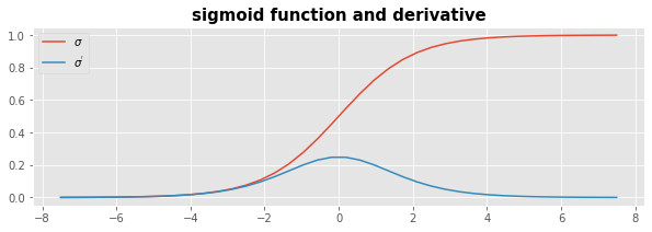
1.2 A mathematical function

During the traning the result of $\boldsymbol{\phi}^T \cdot \mathbf{w}$ will be damped to the interval $[0..1]$ by the sigmoid function $\sigma$.

$$ \sigma = \frac{1}{1 + e^{-x}} $$

The derivative of the sigmoid function $\sigma^{'}$ is given as

$$ \sigma^{'} = \frac{d\sigma}{dx} = \sigma(1-\sigma) $$

def sigmoid(x):  
    return 1.0 / (1.0 + np.exp(-x))

def sigmoid_deriv(x):
    return sigmoid(x)*(1-sigmoid(x))

x = np.linspace(-7.5, 7.5, 40)
with plt.style.context('ggplot'):       
    fig = plt.figure(figsize=(10,3)) ;
    plt.plot(x,sigmoid(x),label=r'$\sigma$'); 
    plt.plot(x,sigmoid_deriv(x),label=r"$\sigma^{'}$");
    plt.title('sigmoid function and derivative', fontsize=15, fontweight='bold'); 
    plt.legend();plt.show()

png

1.3 The way to change the model weights

The basic cycle to train a NN-model is:

Guess some initial values for the model weights $\boldsymbol{w}^n$
Compute with the given training data and the model weights a predicted output value $\Psi_{predicted}^n$. This step is called forward propagation.
Determine how usefull this model prediction was with $\Delta_{Output} = \Psi_{predicted}^n - \Psi_{training \, data}$
Use the error $E = \Delta_{Output}$ in order to find some improved model weights $\boldsymbol{w}^{n+1}$. This step is called backward propagation

The backwardward propagation is the master piece of any NN-algorithm and there are different methods for this task which we will descibe in a later post. For the moment we summarize the core idea:

Given the error $E = \Delta_{Output}$, which of the model weights $\boldsymbol{w}^n$ have contributed to it and how much? An approach is: Large weights contribute largely to the error, small weights only a little. With that rule the error $E = \Delta_{Output}$ is split proportionaly and allocated to the different weights.
If we know the output error and the (estimated) contribution to the error of each weight, in which direction shall we change the weights in order to get an improved model output ? An approach is: we can identify the tendency of the error in dependency of the weights by building its derivative $\frac{\partial E_i}{\partial w_i}$. The direction of improvment is counter this gradient. The weights are therefore updated with

$$ \begin{array}{rclll} \boldsymbol{w}^{n+1} & = & \boldsymbol{w}^{n1} - \alpha \frac{\partial \boldsymbol{E} }{\partial \boldsymbol{w}} \\ & = & \boldsymbol{w}^{n1} - \boldsymbol{\phi}^T \, \cdot \, (\boldsymbol{E} \cdot \sigma^{'}(\Psi_{predicted}^n)) \end{array} $$

Note that it is not straight forward to find this last formula. A basis are the methods of Newton iteration and Gradient descent. An illustrative example of the Gradient descent-method is given in our Post here.

1.4 The training algorithm

The inital values of the model weights are set by random choice in the interval $[0..1]$

#---- initialize the model weights [-1..+1) by random
np.random.seed(1)                         
model_weights = 2 * np.random.random_sample((ny, 1)) - 1
print('inital model_weights.T:', model_weights.T); print()

inital model_weights.T: [[-0.166  0.441 -1.    -0.395 -0.706 -0.815 -0.627]]

The training algorithm runs iteratively through following steps:

predict an output by the model: $\Psi_{predicted}^n = \sigma(\boldsymbol{\phi}^T \cdot \mathbf{w}^n)$
compare the predicted output with the labeled training output data: $\Delta_{Output} = \Psi_{predicted}^n - \Psi_{training \, data}$
find the direction of improvement with the error weighted derivative: $\delta_{weights} = \boldsymbol{\phi}^T \, \cdot \, (\Delta_{Output} \cdot \sigma^{'}(\Psi_{predicted}^n))$
update the weights: $\boldsymbol{w}^{n+1} = \boldsymbol{w}^{n} + \delta_{weights}$
repeat this proces until the change of error $\epsilon$ becomes small: $\epsilon = (\Delta_{Output}^{n+1} - \Delta_{Output}^{n})/\Delta_{Output}^{n+1}$

#---- run the training of the model weights -------------------
dOutput = 4 * np.random.random_sample((nx, 1))                     # ΔOutput = Ψdata - Ψpredicted, initial value

iteration = 0                                                       # running index in the while loop
epsN = 1.1                                                          # norm(error), initial value
epsToler = 3* 10.0**(-5)                                            # error level to stop the while-itertaions
print('{:6d}'.format(iteration),  '{:06.4e}'.format(epsN),  '{:06.4e}'.format(epsToler) ) ;print()

while (epsN > epsToler):                                            # run the model until change of error is small
    W_times_I = np.dot(phi_inp_train, model_weights)                # compute the model training_data * weights
    psi_predicted    = sigmoid(W_times_I)                           # sigmoid function for that
    dO_old = dOutput
    dOutput   = (psi_out_train - psi_predicted)                     # compare the labeled data with the computed result
    gradient  = psi_predicted * (1 - psi_predicted)                 # gradient of the sigmoid function 
    model_weights += np.dot(phi_inp_train.T,  dOutput*gradient)     # update the weights
    epsV = np.abs((dOutput-dO_old)/dOutput)                         # vector of relative error between two iterations
    epsN = np.linalg.norm(epsV)                                     # norm(error)
    if iteration % 10000 == 0: print('{:6d}'.format(iteration),  '{:06.4e}'.format(epsN),  '{:06.4e}'.format(epsN-epsToler) ) 
    iteration += 1

print()
print('{:6d}'.format(iteration),  '{:06.4e}'.format(epsN),  '{:06.4e}'.format(epsN-epsToler) ); print()
print('==> trained model_weights: ', model_weights.T)

     0 1.1000e+00 3.0000e-05

     0 3.0556e+01 3.0556e+01
 10000 1.6818e-04 1.3818e-04
 20000 8.3832e-05 5.3832e-05
 30000 5.5810e-05 2.5810e-05
 40000 4.1822e-05 1.1822e-05
 50000 3.3438e-05 3.4381e-06

 55717 3.0000e-05 -2.1815e-10

==> trained model_weights:  [[12.09  -2.832 -2.746 -5.038 -0.092 -2.835  2.139]]

2. Testing

2.1 Generate testing data

We generate some test input data and output data that we can use to test the NN-model.

#---- initialize the testing arrays
phi_inp_test = np.zeros((nx,ny),dtype=int)
psi_out_test = np.zeros((nx,1),dtype=int)

#---- Generate test input data
np.random.seed(222)
phi_inp_test = np.random.randint(2, size=(nx, ny))
print('phi_inp_test'); print(phi_inp_test); print()

#---- label the test input data as test output data
psi_out_test[:,0] = phi_inp_test[:,0]
print('psi_out_test'); print(psi_out_test); print()

phi_inp_test
[[0 1 1 0 0 0 0]
 [1 0 1 1 1 1 0]
 [0 0 0 1 0 0 0]
 [0 0 1 1 1 1 0]
 [0 1 1 1 1 0 1]
 [1 0 0 1 1 1 1]
 [1 1 0 1 1 0 1]
 [1 1 1 0 1 1 1]
 [1 1 0 0 0 0 0]]

psi_out_test
[[0]
 [1]
 [0]
 [0]
 [0]
 [1]
 [1]
 [1]
 [1]]

2.2 Run the NN model

#---- compute the model: test_data * weights
W_times_I           = np.dot(phi_inp_test, model_weights)                
psi_predicted_raw   = sigmoid(W_times_I)
psi_predicted_round = np.round(psi_predicted_raw ).astype(int) 

np.set_printoptions(precision=3)
print('----------------')
print('raw result      :  psi_predicted =', psi_predicted_raw.T)
print('rounded result  :  psi_predicted =', psi_predicted_round.T)
print('test data       :  psi_out_test  =', psi_out_test.T)

----------------
raw result      :  psi_predicted = [[3.767e-03 7.990e-01 6.448e-03 2.232e-05 1.901e-04 9.981e-01 9.981e-01 9.967e-01 9.999e-01]]
rounded result  :  psi_predicted = [[0 1 0 0 0 1 1 1 1]]
test data       :  psi_out_test  = [[0 1 0 0 0 1 1 1 1]]

3. Error analysis

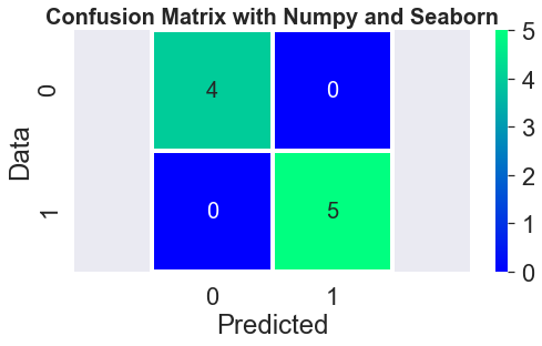
3.1 Confusion matrix with Numpy

We we build some auxiliary arrays as indermediate results to determin the elements of the confusion matrix with vectorized operations.

dPsi = Ψdata - Ψpredicted
LmP = Ψdata * Ψpredicted
LpP = Ψdata + Ψpredicted

print('---- Auxiliary arrays --------------------------')
dPsi  = psi_out_test - psi_predicted_round
LmP   = psi_out_test * psi_predicted_round
LpP   = psi_out_test + psi_predicted_round

print('psi_out_test       ', psi_out_test.T)
print('psi_predicted_round', psi_predicted_round.T)
print('dPsi               ', dPsi.T)
print('LmP                ', LmP.T)
print('LpP                ', LpP.T)

---- Auxiliary arrays --------------------------
psi_out_test        [[0 1 0 0 0 1 1 1 1]]
psi_predicted_round [[0 1 0 0 0 1 1 1 1]]
dPsi                [[0 0 0 0 0 0 0 0 0]]
LmP                 [[0 1 0 0 0 1 1 1 1]]
LpP                 [[0 2 0 0 0 2 2 2 2]]

#---- this methods gives the inidces of aD, LmP, LpP
TP, FP =  np.where(LmP ==1)[1],  np.where(dPsi==-1)[1]
FN, TN =  np.where(dPsi==1)[1],  np.where(LpP ==-0)[1]

ConfusionMatrixNy = np.array([[len(TN), len(FP)],
                             [len(FN), len(TP)]], dtype=int)
print('----- ConfusionMatrixNumpy --------------'); print(ConfusionMatrixNy); print()

with plt.style.context('seaborn'): 
    plt.figure(figsize=(8, 4))
    sn.set(font_scale=2)
    sn.heatmap(ConfusionMatrixNy, annot=True, square=True, annot_kws={"size":20},linewidth=3, cmap='winter')
    plt.xlabel('Predicted'); plt.ylabel('Data')
    plt.axis('equal'); plt.title('Confusion Matrix with Numpy and Seaborn', fontweight='bold',fontsize=20)
    plt.show()

----- ConfusionMatrixNumpy --------------
[[4 0]
 [0 5]]

png

3.2 Confusion matrix with other Python tools

In our Post here we try some other Python tools to evaluate and display the error matrix.

---- Code of the graphics -----

import graphviz as gv

def nn_1():
    d1 = gv.Digraph(format='png',engine='dot')
    d1.attr(rankdir='LR')
    c = ['cornflowerblue','orangered','orange','chartreuse','lightgrey','violet','white']

    d1.node('d1','φ1',    style='filled', color=c[1])
    d1.node('d2','φ2',    style='filled', color=c[0])
    d1.node('d3','....',    style='filled', color=c[5])
    d1.node('d4','φ(n-1)',   style='filled', color=c[4])
    d1.node('d5','φ(n)',   style='filled', color=c[2])
    d1.attr('node', shape='box')
    d1.node('T','Ψ: what is that ?',    style='filled', color=c[3])

    d1.edge('d1','T',label='w1=?') 
    d1.edge('d2','T',label='w2=?')
    d1.edge('d3','T',label='w...=?')
    d1.edge('d4','T',label='w(n-1)=?')
    d1.edge('d5','T',label='w(n)=?')
    return d1
# nn_1()

HealthyNumerics

MachineLearning: A simple but complete artificial Neural Network