Computational Fluid Dynamics : Estimation of the atmospheric surface fluxes

import datetime
from dateutil.relativedelta import relativedelta

import numpy as np
import matplotlib.pyplot as plt
from matplotlib.ticker import MultipleLocator 

float_formatter = lambda x: "%8.2f" % x
np.set_printoptions(formatter={'float_kind':float_formatter})

Solar elevation and irradiation

We give here a procedure to compute the elevation and irraditaion of the sun

def solarRadiation(day):
    Latit = 47.
    rad = np.pi/180.
    NumberOfDay = day.timetuple()[7]                                           # number of days since 1st January
    TMST = day.timetuple()[3]*3600.0 + day.timetuple()[4]* 60.0 + day.timetuple()[5] # True mean solar time in sec
    declin = rad*23.45*np.sin(rad*(280.1 + 0.987*NumberOfDay));                # Declination
    Ht = -np.pi*(43200.0-TMST)/43200.0;                                        # hourley angel                                        
    sinHs =  np.sin(rad*Latit)*np.sin(declin)  \
           + np.cos(rad*Latit)*np.cos(declin)*np.cos(Ht);
    sElevation = np.arctan(sinHs/np.sqrt(1.0-sinHs*sinHs));                    # elevation of sun
    sAzimut = np.cos(declin)*np.sin(Ht)/np.cos(sElevation);                    # azimuth of sun
    kn = NumberOfDay * 2.0*np.pi/365.0;
    I0 = 1353.0 + 45.33*np.cos(kn)   + 0.88* np.cos(2*kn) \
                + 0.005*np.cos(3*kn) + 1.8 * np.sin(kn)   \
                + 0.10 *np.sin(2*kn)+ 0.184* np.sin(3*kn)                       # solar constant
    #S0:= I0 * sinHs                                                            # extraterrestrial radiation
    return I0*sinHs, Ht

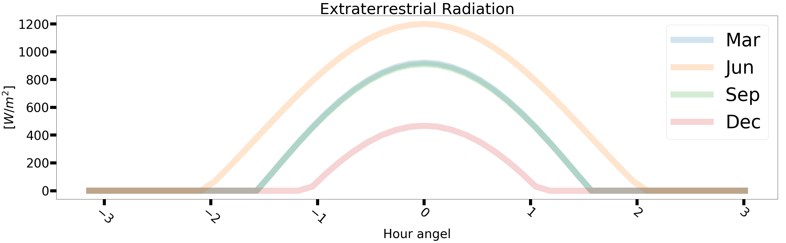
Daily course of solar radition for some selected months

For March, June, September and December of a year we take day 21 and plot the daily corse of the solar extraterestrial raditaion

firstDate = datetime.datetime(2017, 3,21,0,0,0)
lastDate  = datetime.datetime(2018, 3,20,0,0,0)
daySteps  = 1
monthSteps= 3
secSteps  = 0.5 * 3600

dt = datetime.timedelta(seconds = secSteps)

fig = plt.figure(figsize=(42,11)) 
ax1 = fig.add_subplot(111)

date = firstDate
while date <= lastDate:
    nextDay = date.timetuple()[2] + 1
    print('date : ',date)

    d0 = date.replace(hour= 0, minute= 0, second= 0)
    d1 = d0.replace(day = nextDay)    
    Time= np.arange(d0, d1, dt).astype(datetime.datetime)

    A  = np.array( [solarRadiation(Time[t]) for t in range(0,len(Time))] )
    I    = np.maximum(A[:,0], 0.)   #B[B < 0] = 0
    Ht = A[:,1]
    ax1.plot(Ht,I,lw=20, alpha=0.2)

    #date += datetime.timedelta(days=daySteps)
    date += relativedelta(months= monthSteps)

plt.title('Extraterrestrial Radiation',fontsize=50)
plt.xlabel(r'Hour angel', fontsize=40)
plt.ylabel(r'$[W/m^2]$',  fontsize=40)
tickFontsize=40
plt.xticks(fontsize = tickFontsize, rotation=320);
plt.yticks(fontsize = tickFontsize);
plt.tick_params(which='major', length=20, width=10)
plt.legend(['Mar', 'Jun', 'Sep', 'Dec'], loc='upper right',prop={'size': 60})
plt.show()

date :  2017-03-21 00:00:00
date :  2017-06-21 00:00:00
date :  2017-09-21 00:00:00
date :  2017-12-21 00:00:00

png

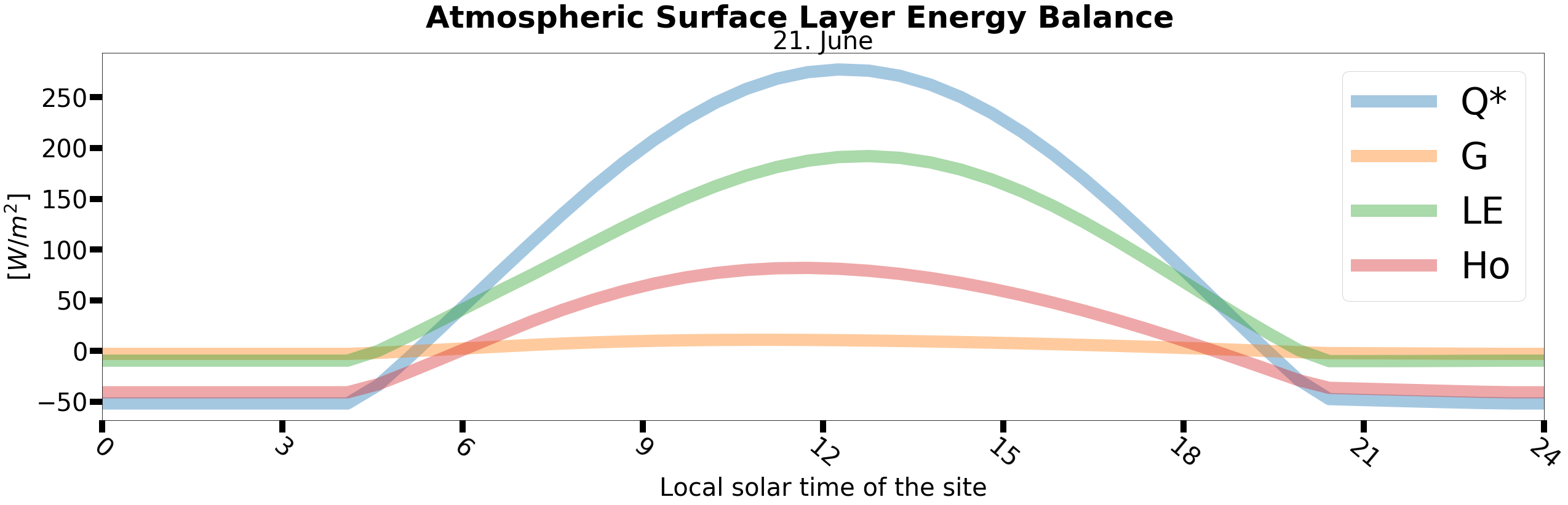
Estimation of the atmospheric surface fluxes

I represents the extraterrestrial radiation at the outer bound of the earth atmosphere. So the transmission through the atmosphere still has to be included. For the moment we ommit this step. To get a first impression of the energy balance at the earth surface we use the following model, which was designed to calculate the energy balance from routine weather data.

 A.A.M.Holtslag, A.P.VanUlden:
 A simple scheme for daytime estimates of the surface fluxes from routine weather data
 J Clim Appl Met 22 (1983) 517-529

 A.P.VanUlden, A.A.M.Holtslag:
 Estimation of atmospheric boundary layer parameters for diffusion applications
 J Cli Appl Met 24 (1985) 1196-1207

We will use I as a parameter for the global raditaion, and we will simulate roughly the temperature T based on I. T shall ondulate between 15 and 25 degree centigrade following the form of I , shifted by 3 hours from noon to 3 p.m.

T = 272. + 15. + 10. * np.roll(I , int((3.*3600.)/secSteps))/max(I)

#----- Energy balance model---------------------------------
def EB2(Gl,T10):
    ''' Input:
    z10:  measurement hight,          z0:  roughness length,
    a  :  albedo,                     Gl:  global radiation,
    T10:  temperature at 10 m,        N :  degree of cloudines
    LEfrac: part of evaporating area
    '''
    #Gl = 750;        T10 = 15. + 273.15;
    z10 = 10.0;        z0 = 0.5;                   
    a   =  0.7;         N = 0.5;                                  
    LEfrac = 0.9;   sigma = 5.67E-8; #Stefan-Boltzmann constant

    #---- radiation balance-----------------------------------
    c1  = 5.31E-13;                c2 = 60.0;     c3 = 0.12;
    T3  = np.exp(3.0*np.log(T10)); T4 = T3*T10;   T6 = T3*T3;
    Qstar = ((1.0-a)*Gl + c1*T6 - sigma*T4 + c2*N)/(1+c3);

    #---- ground heat flux -----------------------------------
    Ag   = 1.0;     S  = np.exp(0.055*(T10-279.0));
    alfa = 1.0;     Ch = 0.38*  ((1.0-alfa)*S + 1.0) / (S+1.0);
    G    = Ag/(4.0*sigma*T3)*Ch*Qstar;

    #---- latent heat flux ---------------------------------------
    LE   =   (S/(S+1.0)*(Qstar-G) + 20.0) * LEfrac

    #---- sensible heat flux  -----------------------------------
    Ho   = Qstar - LE - G;
    return Qstar, G, LE, Ho

We run the model for a mid summer day

d0 = datetime.datetime(2018,6,21,0,0,0)
d1 = datetime.datetime(2018,6,22,0,0,0)
secSteps  = 0.5 * 3600

dt = datetime.timedelta(seconds = secSteps)
Time  = np.arange(d0, d1, dt).astype(datetime.datetime)

A  = np.array( [solarRadiation(Time[t]) for t in range(0,len(Time))] )
I  = np.maximum(A[:,0], 0.)   # A[A< 0] = 0; sets negative values to zero
T  = 272. + 15. + 10. * np.roll(I,int((3.*3600.)/secSteps))/max(I)
Qstar, G, LE, Ho = EB2(I,T)

Graphics

fig = plt.figure(figsize=(42,11)) 
ax1 = fig.add_subplot(111)

t = 24 * (Ht-min(Ht))/(max(Ht)-min(Ht))
ax1.plot(t,Qstar, t,2.*G, t,LE, t,Ho,lw=20, alpha=0.4)

x_majorLoc = MultipleLocator(3)
ax1.set_xlim(0, 24)
ax1.xaxis.set_major_locator(x_majorLoc)

plt.legend(['Q*', 'G', 'LE', 'Ho'], loc='upper right',prop={'size': 60})
plt.suptitle('Atmospheric Surface Layer Energy Balance', fontsize=50, fontweight='bold')
plt.title('21. June',fontsize=40)
plt.xlabel(r'Local solar time of the site', fontsize=40)
plt.ylabel(r'$[W/m^2]$',  fontsize=40)

tickFontsize=40
plt.xticks(fontsize = tickFontsize, rotation=320);
plt.yticks(fontsize = tickFontsize);
plt.tick_params(which='major', length=20, width=10) 
plt.show()

png