Classifying a cloud of points into the corresponding control volumes

In this example we generate 2000 randomly distributed points. We want to know in which control volume of the grid they fall.

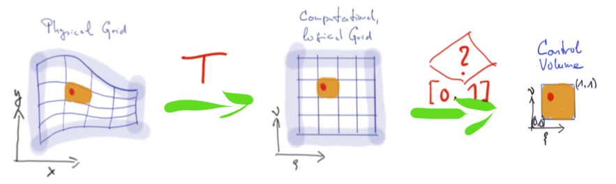
Consider a quadrilateral element with 4 nodes. Sometimes this is called a control volume (in the finite volume community) or a finite element (in the finite element community). We use the finite element (FEM) principle to solve the task in the following steps:

A streched grid in cartesian coordinates can be mapped by transformation \(T\) to a logical or computational grid. The compuational grid is rectangular and each side of the control volumes has the same length, usually 1.
Each control volume is assumed to have its own coordinate system. At the lower left corner is \((0,0)\), at the upper right corner is \((1,1)\).
Each generated point \(P(x,y)\) is expressed by the local coordinates of a control volume, so we get \(P(\xi, \nu)\). If \(\xi\) and \(\nu\) are within the intervall \([0,1]\) the point under consideration belongs to the control volume under consideration.

Some more mathematical details can be found in our post here or in this blog here.

png

import numpy as np
from scipy import optimize

import matplotlib.pyplot as plt
import matplotlib.colors as mclr
from matplotlib import cm
from colorsys import hls_to_rgb

def scale01(z):   #--- transform z to [0 ..1]
    return (z-np.min(z))/(np.max(z)-np.min(z))

def scale11(z):   #--- transform z to [-1 ..1]
    return 2.0*(scale01(z)-0.5)

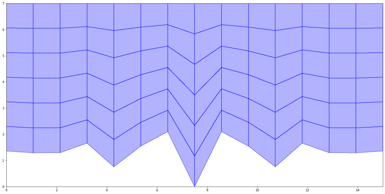
1. Generate a stretched body fitted grid

def get_base_grid(nx,ny):
    ix = np.linspace(0,1,nx)
    iy = np.linspace(0,1,ny)
    x = np.outer(ix,np.ones_like(iy))
    y = np.outer(np.ones_like(ix),iy)
    return ix,iy,x,y

def get_south_boundray(ix):
    sb_case = 1
    if sb_case==1:
        A = 0.5; B = 1.0; C = 5.0; D = 0.25
        Hs = B*np.exp(-(scale11(ix)/A)**2) * D*np.cos(scale01(ix)*C*2.0*np.pi)
        return 0.3*scale01(Hs)

def get_bodyfitted_grid(ix,iy):
    south_boundary = get_south_boundray(ix)
    north_boundary = np.ones_like(south_boundary)
    dY =  north_boundary - south_boundary
    x = np.outer(ix,np.ones_like(iy))
    y = np.outer(dY,iy) + np.outer(south_boundary,np.ones_like(iy)) 
    return x,y

def plot_grid(x,y,z,px,py):
    fig = plt.figure(figsize=(22,11)) 
    ax = fig.add_subplot(111)
    myCmap = mclr.ListedColormap(['white','white'])
    myCmap = mclr.ListedColormap(['blue','lightgreen'])
    ax.pcolormesh(x, y, z, edgecolors='b', lw=1, cmap=myCmap,alpha=0.3)
    ax.scatter(px,py,s=70,c='r')
    #ax.set_aspect('equal')
    plt.show()

#------- main --------------------------------------------
nx,ny = 15,7                       # number of grid points
Lx, Ly = nx, ny                    # length scal of the sides

ix,iy,x,y = get_base_grid(nx,ny)   # generate logical grid
x,y = get_bodyfitted_grid(ix,iy)   # generate physical body fitted grid
x, y = Lx*x, Ly*y

plot_grid(x,y,0*x,[],[])

png

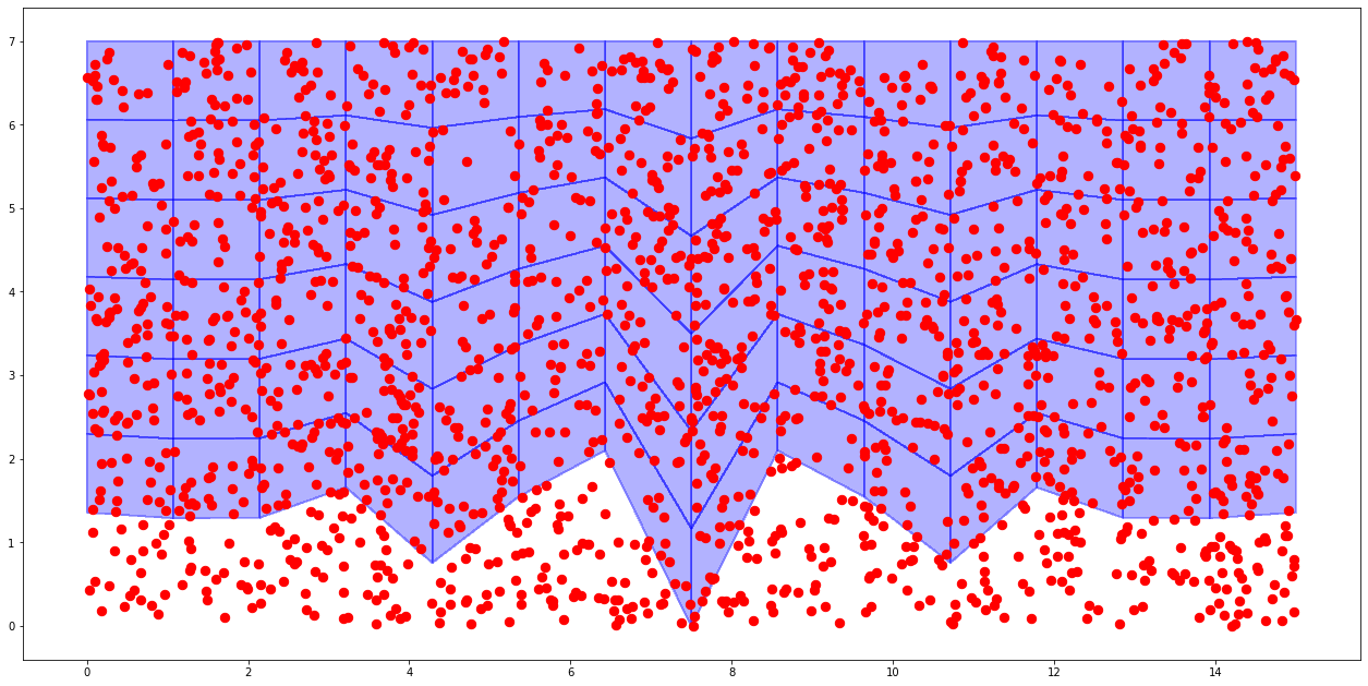
2. Generate a cloud of points

We generate now a cloud of points with the random number generator.

def generate_points(mp,Lx,Ly):
    px,py = Lx*np.random.rand(mp), Ly*np.random.rand(mp)
    return px,py

#------- main --------------------------------------------
MP = 2000                               # number of points
px,py = generate_points(MP,Lx,Ly)
plot_grid(x,y,0*x,px,py)

png

3. Evaluate which points fall in the same control volums of the grid

A point \(P(x,y)\) given in cartesian coordinates must be expressed as \(P(\xi, \nu)\) in logical coordinates. The mapping between \((x,y)\) and \((\xi, \nu)\) is given by

\begin{equation} \begin{array}{lcl} x & = & a_1 + b_1\cdot \xi + c_1\cdot \nu + d_1\cdot \xi\cdot \nu \\ y & = & a_2 + b_2\cdot \xi + c_2\cdot \nu + d_2\cdot \xi\cdot \nu \end{array} \end{equation}

This is a non-linear relation. There is an analytical solution for that. But in our code we use an optimization procedure to determine \((\xi, \nu)\) that is suitable to \((x,y)\).

Once we have \((\xi, \nu)\) we can check whether \(\xi\) and \(\nu\) are within the range \([0..1]\) each. If yes the point is within the area of the control volume under consideration.

def inField(xx,yy):
    if (xx>=0.0 and xx<1.0) and (yy>=0.0 and yy<1.0) : return 1;
    else: return 0

def N0(xj,yj): return (1-xj)*(1-yj)
def N1(xj,yj): return xj*(1-yj)
def N2(xj,yj): return xj*yj
def N3(xj,yj): return (1-xj)*yj

def funcFEMcoord(xj,xp,yp,xc,yc):  # used as function of root-finding 
    return [N0(xj[0],xj[1])*xp[0] + N1(xj[0],xj[1])*xp[1] + 
            N2(xj[0],xj[1])*xp[2] + N3(xj[0],xj[1])*xp[3] - xc ,
            N0(xj[0],xj[1])*yp[0] + N1(xj[0],xj[1])*yp[1] + 
            N2(xj[0],xj[1])*yp[2] + N3(xj[0],xj[1])*yp[3] - yc  ]    

def run_through_cells(x,y,px,py):
    mx,my   = x.shape
    xi,yi = np.zeros_like(px), np.zeros_like(py)
    qx,qy = px.copy(), py.copy()
    Cnpx=np.zeros((mx-1)*(my-1))
    jc = 0
    for ky in range(my-1):
        for kx in range(mx-1):
            px, py = qx.copy(), qy.copy()
            incell = np.zeros_like(px,dtype=int)
            npx = px.shape[0]
            Cnpx[jc] = npx; jc = jc+1
            xc = [x[kx,ky], x[kx+1,ky],x[kx+1,ky+1],x[kx,ky+1]]
            yc = [y[kx,ky], y[kx+1,ky],y[kx+1,ky+1],y[kx,ky+1]]
            plt.scatter(xc,yc,s=80,c='grey',marker='s')
            for jp in range(npx):   # run through the points
                femCoord = optimize.root(funcFEMcoord, [0.5, 0.5],args=(xc,yc,px[jp],py[jp]), method='hybr')
                xi[jp],yi[jp] = femCoord.x
                incell[jp] = inField(xi[jp],yi[jp])
            qx,qy = px[incell==0], py[incell==0]   
            plt.scatter(px[incell==1],py[incell==1],s=100)
    return Cnpx    

#------- main --------------------------------------------
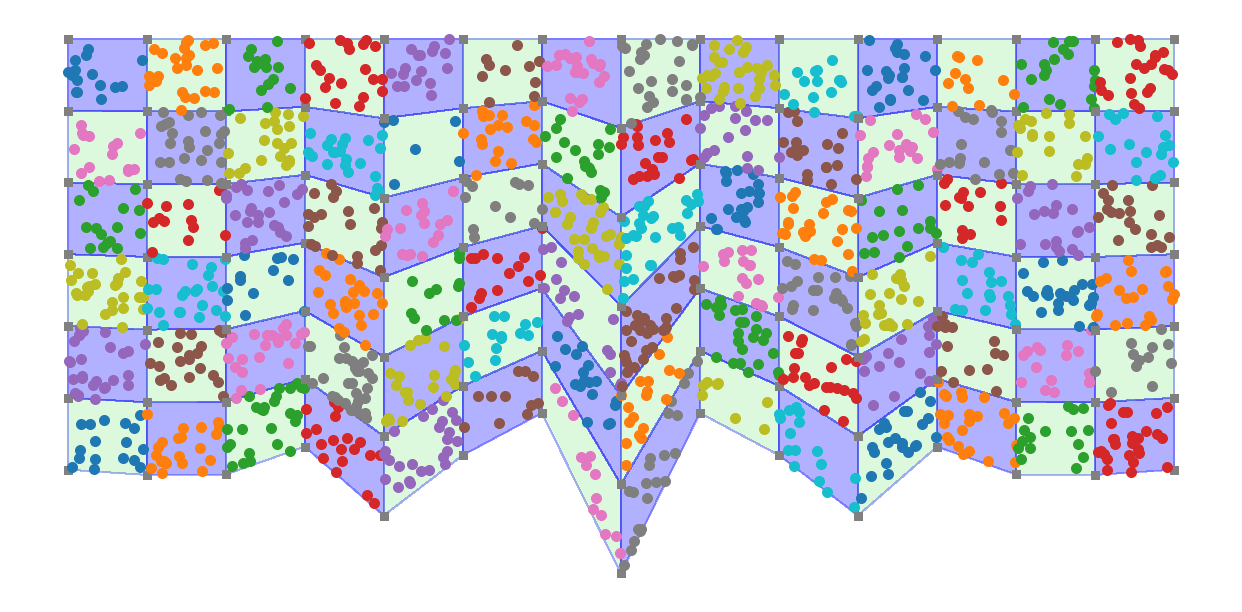
ixn, iyn = np.meshgrid(np.arange(ny,dtype=int),np.arange(nx,dtype=int))
z = (-1)**(ixn+iyn)                                                     # generate a checker board background coloring of the grid

fig = plt.figure(figsize=(22,11))                                       # open the graphical display
ax1 = fig.add_subplot(111)
myCmap = mclr.ListedColormap(['blue','lightgreen'])
ax1.pcolormesh(x, y, z, edgecolors='b', lw=1, cmap=myCmap,alpha=0.3)    # plot the grid
Cnpx  = run_through_cells(x,y,px,py)                                    # determin in whoch control volume each point is
plt.axis('off');plt.show()

png