- So 12 August 2018
- DataScience
- Peter Schuhmacher
- #python, #noise and signal, #data analysis
The distinction between signal and noise is a key issue in data analysis. Early technical applictions include audio and speech processing, sonar, radar and other sensor array processing, spectral density estimation, statistical signal processing, digital image processing, signal processing for telecommunications, control systems, biomedical engineering, seismology, among others.
We will use the following two techniques:
- Convolution, which may include many different kernels
- Nonparametric kernel regression
We have prepared some basics about convolution in an earlier post.
import numpy as np
import pylab as plt
from scipy.interpolate import interp1d
from sklearn.gaussian_process import GaussianProcessRegressor
from sklearn.gaussian_process.kernels import WhiteKernel, ExpSineSquared

np.set_printoptions(linewidth=150, precision=2)
Convolution for data smoothing
A convolution is a way to combine two sequences, f and h, to get a third sequence, y, that is a filtered version of f. The convolution of the sample \(f_n\) with windows \(h\) is formally noted as:
It is the mean of the weighted summation over a window of length WL and \(h\) are the weights. Usually, the sequence h is generated using a window function. Numpy has a number of window functions already implemented: bartlett, blackman, hamming, hanning and kaiser. So, let's use the Kaiser windows withe varying \(\beta\) to filter noisy data.
There are further relations to kernels and kernel smoothers and kernel regression and kernel densitiy estimation
def convolute(yin,beta,WL):
    # WL = 11                  # must be odd: window length
    W2 = int((WL-1)/2)        # half windows lengt
    yLeft = yin[WL-1:0  :-1];
    yRight= yin[  -1:-WL:-1]
    Y = np.r_[yLeft,yin,yRight] # extend the data at the borders
    w = np.kaiser(WL,beta)    # choose the type of wightning in the window
    y = np.convolve(w/w.sum(),Y,mode='valid')
    return y[W2:len(y)-W2]
# input: set the parameter
beta = [2,4,16,32]
beta = [2,16]
WL = 11 # must be odd: window length
#---- generate data ----
nx = 120
ix = np.linspace(0,1,nx) # 0..1
x = 4*(ix-0.2) # x range
y_base = x* np.exp(-x**2) # the base trend
np.random.seed(123)
y = y_base + np.random.randn(nx)*0.2 # add random noise
#---- smooth the data ----
with plt.style.context('fivethirtyeight'):
plt.figure(1, figsize=(20,7))
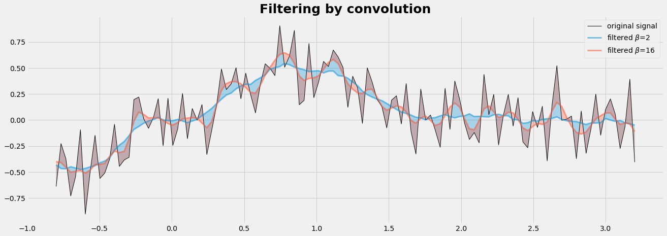
plt.plot(x,y,'k-',label="original signal",lw=1,alpha=0.95)
for b in beta:
ys = convolute(y,b,WL)
plt.plot(x,ys,lw=3, alpha=0.5,label=r'filtered $\beta$=%d ' %(b) )
plt.fill_between(x,ys,y, alpha=0.3)
plt.legend()
plt.title('Filtering by convolution', fontsize=25, fontweight='bold');
plt.show()
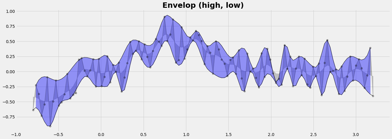
Envelop of the data series
We want to collect the points of 'highs' and 'lows'. We find them at the locations where the slope changes from positive to negative for the 'highs' and vice-versa for the 'lows'. The change of the slope is defined by the 2nd derivative. For the implementation we round the 1st derivative to the sign (= -1 or +1) and compute then the 2nd derivative. We complete both, the line of highs and the line of lows, by cubic interpolation to all points of x.
ys = convolute(y,8,11)              # used for the graphics only
y1 =  np.r_[y[0],y,y[-1]];  x1 = np.r_[x[0],x,x[-1]];
Dy = np.zeros_like(y1);
Dy = np.sign(y1[2:]- y1[1:-1]) - np.sign(y1[1:-1]-y1[0:-2])

yup = y[Dy<0];  xup = x[Dy<0]     # line of highs
ylo = y[Dy>0];  xlo = x[Dy>0]     # line of lows

yupF = interp1d(xup,yup, kind = 'cubic',bounds_error = False)
yloF = interp1d(xlo,ylo, kind = 'cubic',bounds_error = False)
Yup = yupF(x1);
Ylo = yloF(x1);
Graphics
with plt.style.context('fivethirtyeight'):
    plt.figure(1, figsize=(20,7))

    plt.plot(x,y,'ko-', lw=1, alpha=0.3)
    plt.fill_between(x,y,ys, color='k',alpha=0.2)

    plt.plot(x1,Yup, 'k-', lw=1, alpha=0.97)
    plt.plot(x1,Ylo, 'k-', lw=1, alpha=0.97)
    plt.fill_between(x1,Yup,Ylo, color='b',alpha=0.4)

    plt.title('Envelop (high, low)', fontsize=25, fontweight='bold');
    plt.show()
Non-linear regression
Gaussian Kernel Regression is a technique for non-linear regression. The assumption underlying this procedure is that the model can be approximated by a linear function, namely a first-order Taylor series.
Gaussian Processes (GP) are generic supervised learning methods designed to solve regression and probabilistic classification problems. The main features of Gaussian processes are:
- The prediction interpolates the observations (at least for regular kernels).
- The prediction is probabilistic (Gaussian) so that one can compute empirical confidence intervals and decide based on those if one should refit (online fitting, adaptive fitting) the prediction in some region of interest.
- different kernels can be specified. Common kernels are provided, but it is also possible to specify custom kernels.
The GaussianProcessRegressor algorithm is of Bayes type and implements Gaussian processes (GP) for regression purposes. For this, the prior of the GP needs to be specified. The prior mean is assumed to be constant and zero or the training data’s mean.
Kriging in geostatistics is a Gaussian process regression for interpolation which is governed by prior covariances.
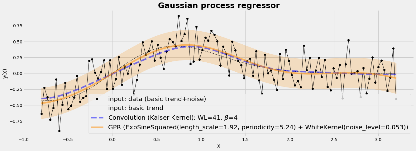
#---- choose the processoer and its kernel
gp_kernel = ExpSineSquared(1.0, 5.0, periodicity_bounds=(1e-2, 1e1))  + WhiteKernel(1e-1)
gpr = GaussianProcessRegressor(kernel=gp_kernel)

#---- run the fitting process
X = x.reshape(-1,1)
gpr.fit(X, y)

#---- predict y using gaussian process regressor
y_gpr, y_std = gpr.predict(X, return_std=True)

#---- predict y using Convolution
b1, WL1 = 4, 41;  ys1 = convolute(y,b1,WL1)
Graphics
with plt.style.context('fivethirtyeight'):
    plt.figure(1, figsize=(20,7))
    plt.plot(x, y, 'ko-', lw=1, label='input: data (basic trend+noise)')
    plt.plot(x, y_base, 'k--', lw=1,  label='input: basic trend')
    plt.plot(x, ys1, 'b--', lw=5, alpha=0.5,  label=r'Convolution (Kaiser Kernel): WL=%d, $\beta$=%d ' %(WL1, b1) )

    plt.plot(X, y_gpr,color='darkorange',lw=5, alpha=0.5,label='GPR (%s)' % gpr.kernel_)
    plt.fill_between(X[:, 0], y_gpr - y_std, y_gpr + y_std, color='darkorange', alpha=0.2)
    plt.xlabel('x'); plt.ylabel('y(x)')

    plt.title('Gaussian process regressor', fontsize=25, fontweight='bold');
    plt.legend(loc="best", scatterpoints=1, prop={'size': 20})
    plt.show()