
- So 08 Juli 2018
- ComputationalFluidDynamics
- Peter Schuhmacher
- #Python, #signal generation, #ECG wave
We generate some basic signals and use convolution and windowing to re-construct ECG waves.
import numpy as np
import matplotlib.pyplot as plt
np.set_printoptions(precision=4,linewidth=160)
Basic Signals
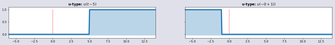
def uSignal(t): return np.array(0.5*np.sign(t) + 0.5,dtype=int)
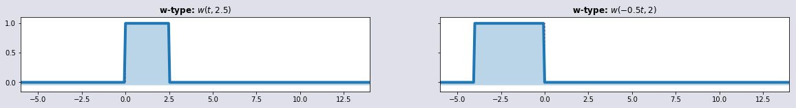
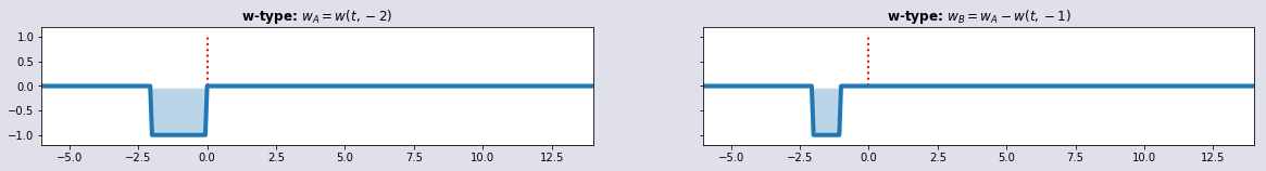
def wSignal(t,dt): return uSignal(t)-uSignal(t-dt)
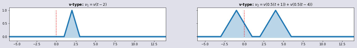
def vSignal(t): return np.maximum(1-np.abs(t),0)
def dSignal(t): DT = t[1]-t[0]; return uSignal(t) - uSignal(t-DT)
def tSignal(t): # trapez
u1 = uSignal(t-0); u2 = uSignal(t-2); u3 = uSignal(t-5); u4 = uSignal(t-7);
t1 = (t-0); t2 = (t-2); t3 = (t-5); t4 = (t-7)
return u1*t1 - u2*t2 - u3*t3 + u4*t4
def sincSignal(t): y1 = np.sinc(t); v1 = vSignal(np.pi/10.0*t); return y1*v1 # sinc = sin(x)/x
def sinquadSignal(t): s = np.sin(t-np.pi/2)**2; w = wSignal(t+np.pi/2,np.pi); return s*w # sin(x)**2
def v_pattern(t,tidx):
V = np.zeros_like(t)
for j in tidx: V = V + vSignal(t-t[j])
return V
def w_pattern(t,tidx,widthW):
W = np.zeros_like(t)
for j in tidx: W = W + wSignal(t-t[j],widthW)
return W
def sinc_pattern(t,tidx):
S = np.zeros_like(t)
for j in tidx: S = S + sincSignal(t-t[j]);
return S
def set_δ(t,ntau):
nt,tmin,tmax = t.shape[0], np.min(t), np.max(t); LT = tmax-tmin; dt = LT/(nt-1)
δτ = 1.0; m_step = int(round(ntau * δτ/dt)) #--- guess the integer 'time step' of the array index
τo = 0; # set-off #--- set the Dirac series
tidx = np.arange(τo,nt,m_step)
t1 = np.zeros_like(t).astype(int); t1[τo:nt:m_step] = 1
return tidx, t1
def scale01(a): return (a-a.min())/(a.max()-a.min()) #--- scale to [0..1]
def scale0(a): return (a-0)/(a.max()-0) #--- scale to [0..1]
def convolution(t,s1,s2):
conv = np.zeros_like(s1)
jt = np.arange(len(s1),dtype=int)
for i,tt in enumerate(t):
conv[i]= np.sum(s1[i-jt]*s2[jt])
return scale01(conv)
Initialize
nt = 301                    # nt grid points
it = np.linspace(0,1,nt)    # dimensionless index
t = 20*(it-0.3)             # time range
Basic signals
u1 = uSignal(t-5); u2 = uSignal(-(t+1)); plot_sig2(t,u1,u2,'u-type: $u(t-5)$','u-type: $u(-(t+1))$')
w1 = wSignal(t,2.5); w2 = wSignal(-0.5*t,2); plot_sig2(t,w1,w2,'w-type: $w(t,2.5)$','w-type: $w(-0.5t,2)$')
w1 = wSignal(t,-2); w2 = wSignal(t,-1); plot_sig2(t,w1,w1-w2,'w-type: $w_A = w(t,-2)$','w-type: $w_B = w_A - w(t,-1)$')
v1 = vSignal(t-2);  v2 = vSignal(0.5*(t+1))+vSignal(0.5*(t-4));
plot_sig2(t,v1,v2,'v-type: $v_1=v(t-2)$','v-type: $v_2=v(0.5(t+1))+v(0.5(t-4))$' )
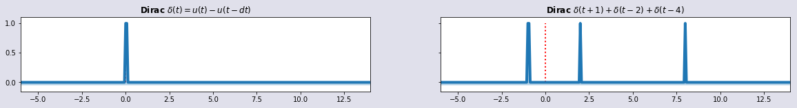
d1=dSignal(t);  dm1=dSignal(t+1); d3=dSignal(t-2); d4=dSignal(t-8); D2=dm1+d3+d4
plot_sig2(t,d1,D2,'Dirac $\delta(t) = u(t)-u(t-dt)$','Dirac $\delta(t+1) + \delta(t-2) + \delta(t-4)$')
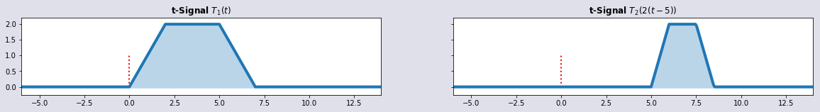
T1 = tSignal(t);  T2 = tSignal(2*(t-5))
plot_sig2(t,T1,T2,'t-Signal $T_1(t)$', 't-Signal $T_2(2(t-5))$')
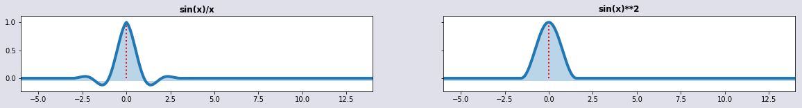
sc = sincSignal(t); sinq=sinquadSignal(t); plot_sig2(t,sc,sinq,'sin(x)/x', 'sin(x)**2')
Signals by convolution
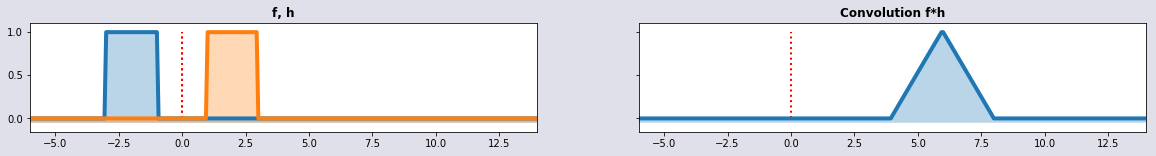
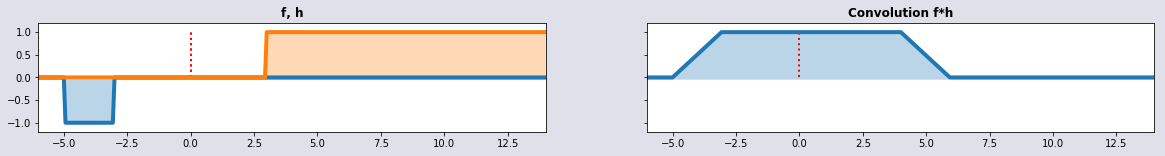
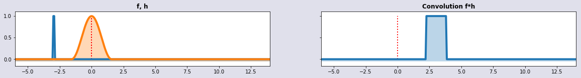
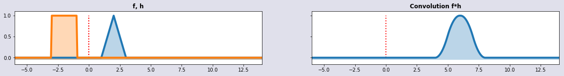
Convolution is a mathematical way of combining two signals to form a third signal. It is the single most important technique in Digital Signal Processing. But it can be used in other areas too. Convolution y at time n of two functions of a continuous variable is in the discrete case defined as:
Convolution can be considered as a generalized form of moving averages. The convolution with the w-signal corresponds to the unweighted (or equi-weighted) mean by a moving window of a certain lenght applied to the original time series. Generalized means that the operator can have more different forms than just an arithmetic mean.
w1 = wSignal(t+3,2); w2 = wSignal(t-1,2); conv = convolution(t,w1,w2); plot_sig4(t,w1,w2,conv,'f, h', 'Convolution f*h')
w1 = wSignal(t+3,-2); w2 = uSignal(t-3); conv = convolution(t,w1,w2); plot_sig4(t,w1,w2,conv,'f, h', 'Convolution f*h')
w1 = dSignal(t+3); w2 = sinq=sinquadSignal(t); conv = convolution(t,w1,w2); plot_sig4(t,w1,w2,conv,'f, h', 'Convolution f*h')
w1 =vSignal(t-2); w2 = wSignal(t+3,2); conv = convolution(t,w1,w2); plot_sig4(t,w1,w2,conv,'f, h', 'Convolution f*h')
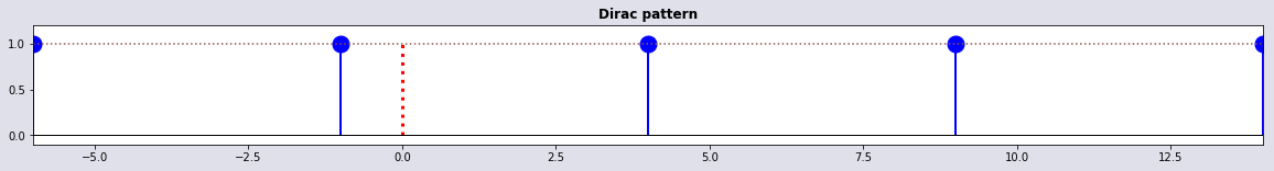
Patterns of signals
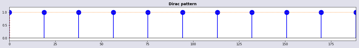
Dirac pattern
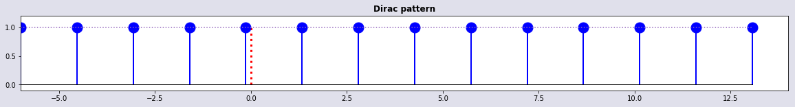
tidx,t1 = set_δ(t,5); plot_stem(t,t[tidx],1 + 0*tidx,'Dirac pattern')
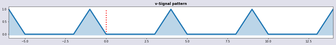
Vp1 = v_pattern(t,tidx); plot_sig1(t,Vp1,'v-Signal pattern')
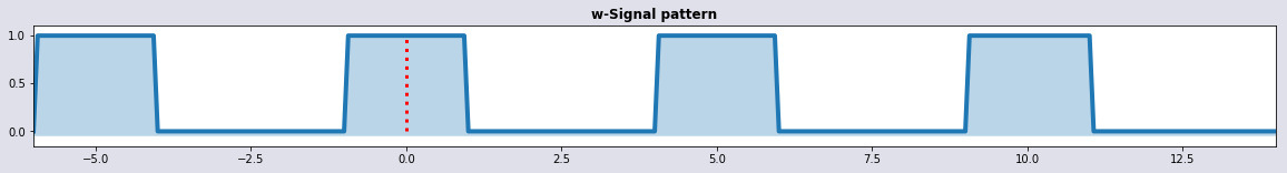
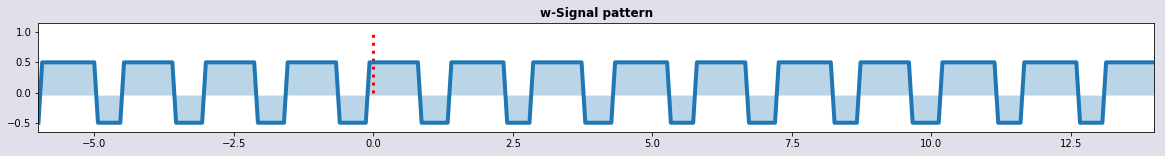
Wp1 = w_pattern(t,tidx,2); plot_sig1(t,Wp1,'w-Signal pattern')
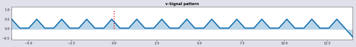
tidx,t1 = set_δ(t,1.5);    plot_stem(t,t[tidx],1 + 0*tidx,'Dirac pattern')
Vp2 = v_pattern(t,tidx);   plot_sig1(t,Vp2-0.5,'v-Signal pattern')
Wp2 = w_pattern(t,tidx,1); plot_sig1(t,Wp2-0.5,'w-Signal pattern')
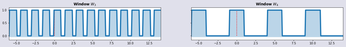
Windowing
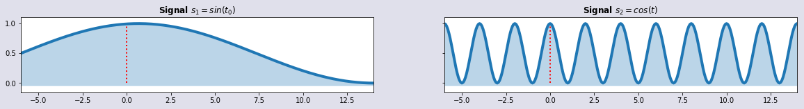
In signal processing and statistics, a window function is a mathematical function that is zero-valued outside of some chosen interval. Mathematically, another function is elementwise multiplied by a window function. The product is zero-valued outside the interval: all that is left is the part where they overlap, so we get the "view through the window".
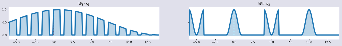
s1 = 0.5*(1 + np.sin(1.5*it*np.pi))
s2 = 0.5*(1 + np.cos(1.0* t*np.pi))
plot_sig2(t,s1,s2,'Signal $s_1= sin(t_0) $', 'Signal $s_2=cos(t)$')
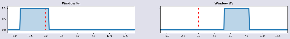
w1 = wSignal(t+4,4.5); w2 = wSignal(t-4,4.0);
plot_sig2(t,w1, w2, 'Window $W_1$','Window $W_2$')
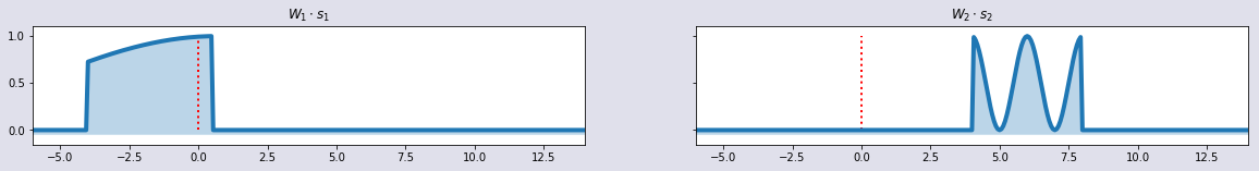
plot_sig2(t,w1*s1,w2*s2,'$W_1 \cdot s_1$','$W_2\cdot s_2$')
plot_sig2(t,Wp2,   Wp1,   'Window $W_3$',   'Window $W_4$')
plot_sig2(t,Wp2*s1,Wp1*s2,'$W_3 \cdot s_1$','$W4 \cdot s_2$')
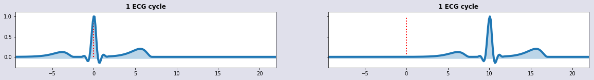
Heart beat (ECG wave)
A description in detail about
- P wave
- Q-R-S complex
- T wave
can be found here .
The single heart beat signal
#----- define t --------------------
nt, it, thor  = 301, np.linspace(0,1,nt), 5   # nt grid points # dimensionless index # time horizon
t = thor*2*np.pi*(it-0.3)                     # time range

#----- 1 heart beat cycle
HB1 = HeartBeatSignal(t); HB2 = HeartBeatSignal(t-10)
plot_single(t,HB1,0*HB1, 0*HB1)
plot_sig2(t,HB1,HB2,'1 ECG cycle', '1 ECG cycle')
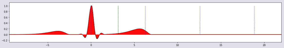
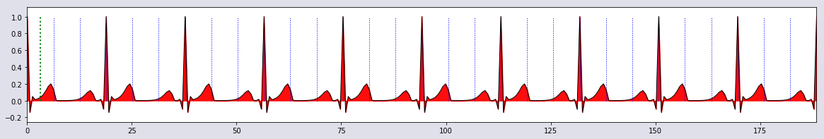
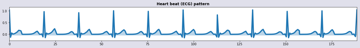
The heart beat (ECG) pattern
def HeartBeatSignal(t):
    v1width= 0.2*np.pi;  v1shift = 0.05*np.pi
    y1 = np.sinc(2.0*t); v1 = vSignal(v1width*(t-v1shift)); yv1 =y1*v1
    S0 = scale0(v1*y1)
    sf1= 1.5*np.pi; A1 = 0.12; sq1 = A1*sinquadSignal(np.exp(0.5*(t+sf1))- np.pi/2)
    sf2= 1.5*np.pi; A2 = 0.20; sq2 = A2*sinquadSignal(np.exp(0.5*(t-sf2))- np.pi/2)
    return sq1+S0+sq2

def HeartBeat_pattern(t,tidx):
    V = np.zeros_like(t)
    for j in tidx: V = V + HeartBeatSignal(t-t[j])
    return V

def ar(u): np.random.seed(1234); return u*(1+0.080*np.random.randn(nt))
def tr(u): np.random.seed(1234); return u*(1+0.001*np.random.randn(nt))

#----- define t --------------------
nt, it, thor  = 301, np.linspace(0,1,nt), 30   # nt grid points # dimensionless index # time horizon
t = thor*2*np.pi*(it-0)                        # time range

#----- build ECG pattern -------------
tidx,t1 = set_δ(t,3*2*np.pi);    plot_stem(t,t[tidx],1 + 0*tidx,'Dirac pattern')
hbp = HeartBeat_pattern(t,tidx);

#---- plot it ----------------------
plot_single(t,hbp,0*t,0*t)
plot_sig1(tr(t),ar(hbp),'Heart beat (ECG) pattern') # with small random cosmetics
Grafics
def plot_sig1(t,y1,title1):
    fig, (ax1) = plt.subplots(1, 1, sharey=True,figsize=(20,2),facecolor=('#e0e0eb'))
    nt,tmin, tmax = t.shape[0], np.min(t), np.max(t)
    ax1.set_xlim([tmin, tmax]);
    g_zero = -0.05;
    ax1.plot(t,y1,lw=4); ax1.fill_between(t, g_zero, y1, alpha=0.3)
    ax1.vlines(0,0,1,'r',linestyles='dotted',lw=3)
    ax1.set_title(title1,fontweight='bold'); ax1.margins(0, 0.1)
    plt.show()

def plot_sig2(t,y1,y2,title1,title2):
    fig, (ax1,ax2) = plt.subplots(1, 2, sharey=True,figsize=(20,2),facecolor=('#e0e0eb'))
    nt,tmin, tmax = t.shape[0], np.min(t), np.max(t)
    g_zero = -0.05;
    ax1.set_xlim([tmin, tmax]);
    ax1.plot(t,y1,lw=4); ax1.fill_between(t, g_zero, y1, alpha=0.3)
    ax1.vlines(0,      0,1,'r',linestyles='dotted',lw=2)
    ax1.set_title(title1,fontweight='bold'); ax1.margins(0, 0.1)
    ax2.set_xlim([tmin, tmax]);
    ax2.plot(t,y2,lw=4); ax2.fill_between(t, g_zero, y2, alpha=0.3)
    ax2.vlines(0,      0,1,'r',linestyles='dotted',lw=2)
    ax2.set_title(title2,fontweight='bold'); ax2.margins(0, 0.1)
    plt.show()

def plot_sig3(t,y1, title):
    fig, (ax1) = plt.subplots(1, 1, sharey=True,figsize=(25,2),facecolor=('#e0e0eb'))
    nt,tmin, tmax = t.shape[0], np.min(t), np.max(t)
    ax1.set_xlim([tmin, tmax]);
    g_zero = -0.05;
    ax1.plot(t,y1,lw=1);
    ax1.fill_between(t, g_zero, y1, alpha=0.3)

    ax1.vlines(0,      0,1,'r',linestyles='dotted',lw=3)
    ax1.vlines(  np.pi,0,1,'g',linestyles='dotted',lw=2)
    for ih in range(thor):
        ax1.vlines(ih*2*np.pi,0,1,'b',linestyles='dotted',lw=1)
    ax1.margins(0, 0.1)
    plt.show()


def plot_sig4(t,y0,y1,y2,title1,title2):
    fig, (ax1,ax2) = plt.subplots(1, 2, sharey=True,figsize=(20,2),facecolor=('#e0e0eb'))
    nt,tmin, tmax = t.shape[0], np.min(t), np.max(t)
    g_zero = -0.05;
    ax1.set_xlim([tmin, tmax]);
    ax1.plot(t,y0,lw=4); ax1.fill_between(t, g_zero, y0, alpha=0.3)
    ax1.vlines(0,      0,1,'r',linestyles='dotted',lw=2)

    ax1.set_xlim([tmin, tmax]);
    ax1.plot(t,y1,lw=4); ax1.fill_between(t, g_zero, y1, alpha=0.3)
    ax1.vlines(0,      0,1,'r',linestyles='dotted',lw=2)

    ax1.set_title(title1,fontweight='bold'); ax1.margins(0, 0.1)
    ax2.set_xlim([tmin, tmax]);
    ax2.plot(t,y2,lw=4); ax2.fill_between(t, g_zero, y2, alpha=0.3)
    ax2.vlines(0,      0,1,'r',linestyles='dotted',lw=2)
    ax2.set_title(title2,fontweight='bold'); ax2.margins(0, 0.1)
    plt.show()

def plot_stem(t,x,y,title):
    nt,tmin, tmax = t.shape[0], np.min(t), np.max(t)
    fig, (ax1) = plt.subplots(figsize=(20,2),facecolor=('#e0e0eb'))
    ax1.set_xlim([tmin, tmax]);  ax1.set_ylim([-0.1, 1.2])   # Grösse der Grafik fixieren (ax = Links)
    markerline, stemline, baseline = plt.stem(x, y, '-')
    plt.setp(baseline, 'color', 'k', 'linewidth', 1)
    plt.setp(stemline, 'color', 'b', 'linewidth', 2)
    plt.setp(markerline, 'color', 'b', 'markersize', 15)
    ax1.vlines(0,0,1,'r',linestyles='dotted',lw=3)
    plt.title(title,fontweight='bold')
    plt.plot(x,y,':')
    plt.show()

def plot_single(t,y1,y2,y3):
    fig, (ax1) = plt.subplots(1, 1, sharey=True,figsize=(20,3),facecolor=('#e0e0eb'))
    nt,tmin, tmax = t.shape[0], np.min(t), np.max(t)
    ax1.set_xlim([tmin, tmax]);
    g_zero = -0.0;
    lw=1
    ax1.plot(t,y1,lw=lw,color='k');
    #ax1.plot(t,y2,lw=lw);
    #ax1.plot(t,y3,lw=lw);
    ax1.fill_between(t, g_zero, y1, color='r',alpha=0.95)

    ax1.vlines(0,      0,1,'r',linestyles='dotted',lw=3)
    ax1.vlines(  np.pi,0,1,'g',linestyles='dotted',lw=2)
    for ih in range(thor):
        ax1.vlines(ih*2*np.pi,0,1,'b',linestyles='dotted',lw=1)
    ax1.margins(0, 0.1)
    plt.show()