We compare 4 numerical principles that have smoothing and/or time marching properties and show the similarities between them.

Let's look at the 1-dimensional case first and let's assume that we have a data series with the connectivity given by the following images. We will use the local compass notation where the central point under consideration is denoted with P and the neighbouring points to the right and to the left with W (=west) and E (=east).

d1

svg

Moving Average = Diffusion = Markov Chain = Monte Carlo

Moving average | A common and simple schema for smoothing is the moving average with a filter length of 3 elements and with weights \((1, 2, 1)/4\):

\begin{equation} \begin{array}{lcl} T^1_P & = & (T^0_W + 2T^0_P + T^0_E)/4 \\ & = & 0.25\,T^0_W + 0.5\,T^0_P + 0.25\,T^0_W \end{array} \end{equation}

Diffusion | Difffusion is a physcical concept and the smoothing properties to reduce differences are well known. A formal similarity to the moving avarage is given with the discretisation of the time dependent diffusion equation. If we scale the term \((\Delta x)^2 / \Delta t\) to 4 then we get:

\begin{equation} \begin{array}{rcl} T_t & = & \nabla^2 T \\ T^1_P - T^0_P & = & (T^0_W - 2T^0_P + T^0_E)\,\Delta t / (\Delta x)^2\\ & = & 0.25\,T^0_W - 0.5\,T^0_P + 0.25\,T^0_W \\ T^1_P & = & 0.25\,T^0_W + 0.5\,T^0_P + 0.25\,T^0_W \\ \end{array} \end{equation}

Markov chain | The stencil as given by the discretisised difffusion equation can be used the build the complete system matrix D which has the structure

 [[1.   0.   0.   0.   0.   0.   0.   0.  ]
  [0.25 0.5  0.25 0.   0.   0.   0.   0.  ]
  [0.   0.25 0.5  0.25 0.   0.   0.   0.  ]
  [0.   0.   0.25 0.5  0.25 0.   0.   0.  ]
  [0.   0.   0.   0.25 0.5  0.25 0.   0.  ]
  [0.   0.   0.   0.   0.25 0.5  0.25 0.  ]
  [0.   0.   0.   0.   0.   0.25 0.5  0.25]
  [0.   0.   0.   0.   0.   0.   0.   1.  ]]

We have now the mathematical form of a Markov chain where status \(T^0\) changes to the new status \(T^1\) with

\begin{equation} \begin{array}{rcl} T^0 & \xrightarrow{\mathbf{D}} & T^1 \\ & & T^1 = \mathbf{D} \cdot T^0 \\ \end{array} \end{equation}

Monte Carlo, MC | We can use the diffusion approach once more and imagine that a physical particle randomly stays either at its starting point P or moves to one of the neighbouring points W or E. If we assume that the particle stays with probability \(p=0.5\) at the position where it is and changes with probability \(p=0.25\) to one of the neighbouring points, then we have the probabilistic counter part to the discretizised partial differential equation of diffusion.

d2

svg

Example: Diffusion vs Moving Average

In the following example we use the diffusion equation in the stationary form und resolve for the central point \(P\) by a Gauss-Seidel principle. For simplicity we use \(\Delta x = 1\).

\begin{equation} \begin{array}{rcl} \nabla^2 T & = & 0 & \text{Diffusion without any sinks or sources}\\ & = & (T^0_W - 2T^0_P + T^0_E)\, / \,(\Delta x)^2 & \text{discretized form} \\ T^0_P & = & (T^0_W + T^0_E)\, / \, 2 & \text{resolve for the central point under consideration}\\ T^1_P & := & (T^0_W + T^0_E)\, / \, 2 & \text{algorithmic Gauss-Seidel form}\\ \end{array} \end{equation}

The last equation is the numerical schema which is one possibility to solve the system equation by the Gauss-Seidel principle. The algorithmic formula of the diffusion is now a moving average with 2 elements only. This is more efficient for smoothing than the formula for the moving average with 3 elements. Both algorithms converge to the same solution, which is a straight line between the boundary points.

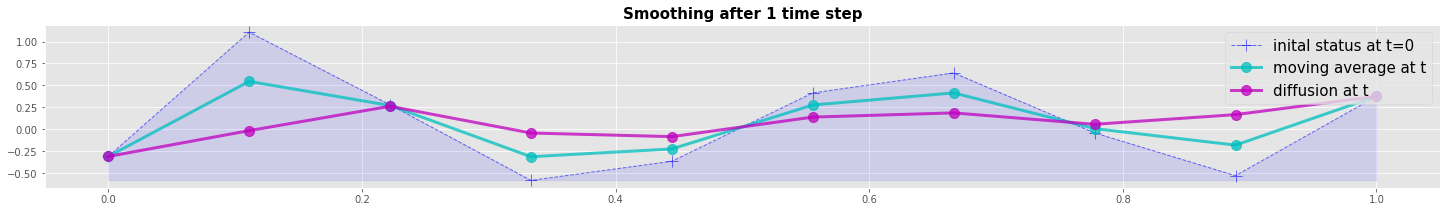
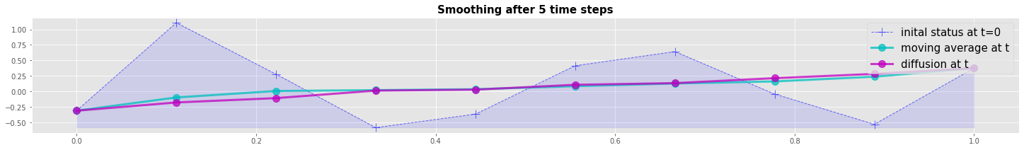
Numerical example: Diffusion vs Moving Average

We compare the Diffusion with the Moving Average method by a numerical example. Both methods are explicite forwad in time. The resulting plot shows that the diffusion method is a more efficient smoother after the first time step. But both methods converge to the same result after 5 time steps.

import numpy as np
import matplotlib.pyplot as plt
np.set_printoptions(linewidth=200)

def scale(a): return (a-np.min(a))/(np.max(a)-np.min(a))

def generate_data_1(case,N):
    np.random.seed(seed=1234)
    x = np.linspace(0,N-1,N);
    if case=='A': z = 12*(scale(x)-0.5); y = np.exp(-z*z);
    if case=='B': y = np.sin(4*np.pi*scale(x))
    if case=='C': y = np.cumsum(np.random.randn(N))
    if case=='R': y = 0*x; n4=N//4; y[n4:-n4]=1
    x = np.linspace(0,1,N)
    return x, y + np.random.random(y.shape)-0.5

def MovingAverage(Z):
    nx= Z.shape[0]
    jxm = slice(0,nx-2);  jx = slice(1,nx-1); jxp = slice(2,nx)   
    Za = Z.copy()  
    Za[jx] = (Z[jxp] + 2.0*Z[jx] + Z[jxm])/4
    return Za

def Diffusion(Z):
    nx= Z.shape[0]
    jxm = slice(0,nx-2);  jx = slice(1,nx-1); jxp = slice(2,nx)   
    Zxx = Z.copy()  
    Zxx[jx] =  (Z[jxp]  + Z[jxm])/2
    return Zxx

def plot_line_1(x,v0,v1,v2,title):
    fig, ax = plt.subplots(figsize=(25,3))
    vmin = v0.min()
    ax.plot(x,v0, 'b+--', ms=12, lw=1, alpha=0.55, label='inital status at t=0')
    ax.plot(x,v1, 'co-', ms=10, lw=3, alpha=0.75, label='moving average at t')
    ax.plot(x,v2, 'mo-', ms=10, lw=3, alpha=0.75, label='diffusion at t')
    ax.fill_between(x,v0,vmin,alpha=0.1,color='b')
    ax.legend(loc=1,prop={'size': 15})
    plt.title(title, fontweight='bold', fontsize=15)
    plt.show()

#------------- main -----------------------------------------
Nn = 10
x,v0 = generate_data_1('B',Nn)  #B, 10

v1 = MovingAverage(v0)
v2 = Diffusion(v0)
with plt.style.context('ggplot'):  
    plot_line_1(x,v0,v1,v2, 'Smoothing after 1 time step')

for k in range(5):
    v1 = MovingAverage(v1)
    v2 = Diffusion(v2)

with plt.style.context('ggplot'):  
    plot_line_1(x,v0,v1,v2, 'Smoothing after 5 time steps')

png

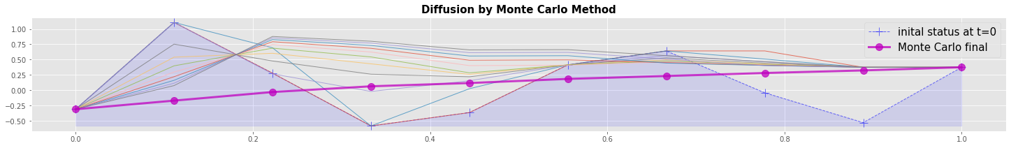
Numerical example: Diffusion by Monte Carlo method

Ther are different possibilities to implement a Monte Carlo method for diffusion. In this example we imagine, that the given data points are particles that have the given temperature. The particles can move to the right and to the left but will not change the temperature. Collisions or friction with other particles are not considered.

We run Nt=1000 timesteps where the status changes from \(v_t\) to \(v_{t+1}\). At each change \(v_{t+1}\) decides whether it takes at position P the same value \(v(P)_t\) with probability \(p=0.5\) or whether it takes the value of one of the neighbouring points \(v(W)_t\) or \(v(E)_t\) with probability \(p=0.25\) each. We sum up all \(v_t\) elementwise and build the mean over all timestpes Nt as final result.

In the graphical output we can recognize a smoothing of the major differences during the first few time steps. The steady state is reached with a lower convergence rate.

def plot_line_2(x,v0,v1,v2,title):
    fig, ax = plt.subplots(figsize=(25,3))
    vmin = v0.min()
    ax.plot(x,v0, 'b+--', ms=12, lw=1, alpha=0.55, label='inital status at t=0')
    ax.plot(x,v1, 'co-', ms=10, lw=3, alpha=0.75, label='moving average at t')
    ax.plot(x,v2, 'mo-', ms=10, lw=3, alpha=0.75, label='diffusion at t')
    ax.fill_between(x,v0,vmin,alpha=0.1,color='b')
    ax.legend(loc=1,prop={'size': 15})
    plt.title(title, fontweight='bold', fontsize=15)
    plt.show()



#------------- main -----------------------------------------
Nt = 1000       # number of iterations
Nmod = 20    # modulo for printing
Nn = 10      # number of points

x,v0 = generate_data_1('B',Nn)
vAll = np.zeros(Nn)
ind1, ind2 = np.arange(Nn),np.arange(Nn) 

with plt.style.context('ggplot'):
    fig, ax = plt.subplots(figsize=(25,3))
    vmin = v0.min()
    ax.plot(x,v0, 'b+--', ms=12, lw=1, alpha=0.55, label='inital status at t=0')
    ax.fill_between(x,v0,vmin,alpha=0.1,color='b')        
    for jt in range(Nt):
        dind = np.random.choice([-1,0,1], Nn, p=[0.25, 0.50, 0.25])
        dind[0], dind[Nn-1] = 0, 0
        ind2 = ind1 + dind
        v1 = v0[ind2]
        vAll = vAll + v1
        #if (jt-1)%Nmod == 0:
        if jt <= 10:
            print('plot at jt=',jt)
            vPlot = vAll/(jt+1)
            ax.plot(x,vPlot,  ms=1, lw=1, alpha=0.75)
        v0 = v1.copy()

    vAll = vAll/Nt
    ax.plot(x,vAll, 'mo-', ms=10, lw=3, alpha=0.75, label='Monte Carlo final')
    plt.title('Diffusion by Monte Carlo Method', fontweight='bold', fontsize=15)
    ax.legend(loc=1,prop={'size': 15})
    plt.show()

plot at jt= 0
plot at jt= 1
plot at jt= 2
plot at jt= 3
plot at jt= 4
plot at jt= 5
plot at jt= 6
plot at jt= 7
plot at jt= 8
plot at jt= 9
plot at jt= 10

png

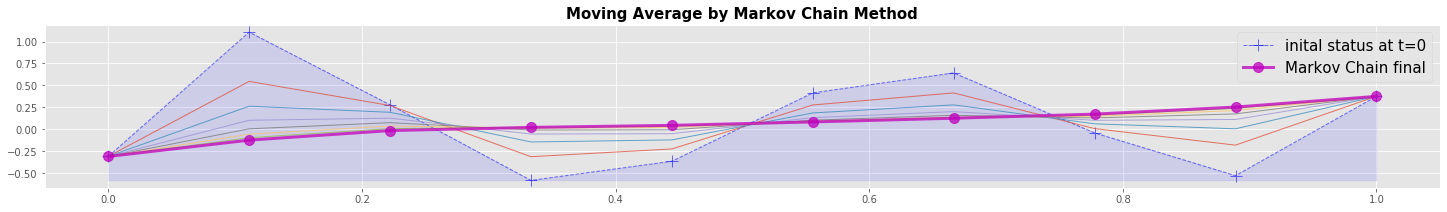
Numerical example: Markov Chain method

A Markov chain changes status \(T^0\) to the new status \(T^1\) with matrix \(M\)

\begin{equation} \begin{array}{rcl} T^0 & \xrightarrow{\mathbf{M}} & T^1 \\ & & T^1 = \mathbf{M} \cdot T^0 \\ \end{array} \end{equation}

Matrix \(M\) can express different things, e.g. Moving Avaerage (MA) or Diffusion (D). The local stencils are:

\begin{equation} \begin{array}{rcl} T^1_P & = & (0.25T^0_W - 0.5T^0_P + 0.25T^0_E) & \text{Diffusion, explicite discretized form} \\ T^1_P & = & (0.25T^0_W + 0.5T^0_P + 0.25T^0_E) & \text{Moving Average } \\ \end{array} \end{equation}

We get the global system matrix M by bringing all the local stencils together. For the Moving Average matrix \(M\) is:

 [[1.   0.   0.   0.   0.   0.   0.   0.  ]
  [0.25 0.5  0.25 0.   0.   0.   0.   0.  ]
  [0.   0.25 0.5  0.25 0.   0.   0.   0.  ]
  [0.   0.   0.25 0.5  0.25 0.   0.   0.  ]
  [0.   0.   0.   0.25 0.5  0.25 0.   0.  ]
  [0.   0.   0.   0.   0.25 0.5  0.25 0.  ]
  [0.   0.   0.   0.   0.   0.25 0.5  0.25]
  [0.   0.   0.   0.   0.   0.   0.   1.  ]]

For the Diffusion the \(0.5\) in the diagonal would become \(-0.5\). The elements with \(1.\) make shure that the boundary values do not change.

In the graphical output we can recognize that the Moving Average converges within a few timesteps close to steady state. At the end the Markov Chain is a different algorithmic form of programming the Moving Average on the data vector as shown above.

def MarkovMatrix_fixed_BC(N):
    D =  np.diag(2.0*np.ones(N))       \
       + np.diag(    np.ones(N-1),  1) \
       + np.diag(    np.ones(N-1), -1)
    D = D/4.0
    D[ 0, 0]=1;  D[ 0, 1]=0
    D[-1,-1]=1;  D[-1,-2]=0
    return D
#------------- main -----------------------------------------
Nt = 7                                    # number of iterations
Nmod = 20                                 # modulo for printing
Nn = 10                                   # number of data points

M = MarkovMatrix_fixed_BC(Nn)              # set up Markov Matrix with fixed boundary conditions
print('-----------------------------------------------------')
print("Markov Transition Matrix M:"); 
print('-----------------------------------------------------')
print(M); print('-----------------------------------------------------')
x,v0 = generate_data_1('B',Nn)             # initialize the data vector


with plt.style.context('ggplot'):
    fig, ax = plt.subplots(figsize=(25,3))
    vmin = v0.min()
    ax.plot(x,v0, 'b+--', ms=12, lw=1, alpha=0.55, label='inital status at t=0')
    ax.fill_between(x,v0,vmin,alpha=0.1,color='b')        
    for jt in range(Nt):
        v1 = np.dot(M,v0)
        ax.plot(x,v1, ms=1, lw=1, alpha=0.75)
        v0 = v1.copy()

    vAll = vAll/Nt
    ax.plot(x,v0, 'mo-', ms=10, lw=3, alpha=0.75, label='Markov Chain final')
    plt.title('Moving Average by Markov Chain Method', fontweight='bold', fontsize=15)
    ax.legend(loc=1,prop={'size': 15})
    plt.show()

-----------------------------------------------------
Markov Transition Matrix M:
-----------------------------------------------------
[[1.   0.   0.   0.   0.   0.   0.   0.   0.   0.  ]
 [0.25 0.5  0.25 0.   0.   0.   0.   0.   0.   0.  ]
 [0.   0.25 0.5  0.25 0.   0.   0.   0.   0.   0.  ]
 [0.   0.   0.25 0.5  0.25 0.   0.   0.   0.   0.  ]
 [0.   0.   0.   0.25 0.5  0.25 0.   0.   0.   0.  ]
 [0.   0.   0.   0.   0.25 0.5  0.25 0.   0.   0.  ]
 [0.   0.   0.   0.   0.   0.25 0.5  0.25 0.   0.  ]
 [0.   0.   0.   0.   0.   0.   0.25 0.5  0.25 0.  ]
 [0.   0.   0.   0.   0.   0.   0.   0.25 0.5  0.25]
 [0.   0.   0.   0.   0.   0.   0.   0.   0.   1.  ]]
-----------------------------------------------------

png

Filtering by implicit partial differential equations or by statistical methods

All the proposed methods use an explicite forward timestep. This in so far not satisfying as the final result depends on how many time steps are chosen. There are more sophisticated methods which use implicit partial differential equations as filtering schemes. In a separate article we will present three approaches:

Raymond and Garder have developed an implicit method in connection with numerical meteorological studies which are meanwhile widely used in computational aeroacoustics and image processing.
we will present our approach which uses both the initial data as driving force with a generating property and the filter with a smoothing property. The solution is a steady state between the generating und the smoothing forces.
a Gaussian processes (GP) for regression purposes as a statistical method. For this, the prior of the GP needs to be specified. A regression can be considered as a smoothing of a data set.

Appendix: Graphics with graphviz

import graphviz as gv
def plotMarkovModel():
    d1 = gv.Digraph(format='png',engine='dot')
    c = ['cornflowerblue','orangered','orange','chartreuse','lightgrey']
    #d1.node('A','A (healthy)', style='filled', color=c[0])
    #d1.node('B','B (infected)',style='filled', color=c[1])
    d1.node('0','0',    style='filled', color=c[4])
    d1.node('P','P',    style='filled', color=c[1])
    d1.node('W','W',    style='filled', color=c[0])
    d1.node('E','E',    style='filled', color=c[3])
    d1.node('n','n',    style='filled', color=c[4])

    d1.edge('0','0',label=''); d1.edge('0','1',label=''); 
    d1.edge('1','1',label=''); d1.edge('1','0',label=''); d1.edge('1','...',label='')
    d1.edge('...','...',label=''); d1.edge('...','1',label=''); d1.edge('...','W',label='')    
    d1.edge('W','W',label=''); d1.edge('W','...',label=''); d1.edge('W','P',label='w+')
    d1.edge('P','P',label=''); d1.edge('P','W',label='w-'); d1.edge('P','E',label='e-')
    d1.edge('E','E',label=''); d1.edge('E','P',label='e+'); d1.edge('E','....',label='')
    d1.edge('....','....',label=''); d1.edge('....','n-1',label=''); d1.edge('....','E',label='')     
    d1.edge('n-1','n-1',label=''); d1.edge('n-1','....',label=''); d1.edge('n-1','n',label='')
    d1.edge('n','n',label=''); d1.edge('n','n-1',label=''); 
    d1.attr(rankdir='LR')
    return d1
d1 = plotMarkovModel()
#d1.render('img/mamo1', view=True)
d1

svg

def plotMCMC():
    d1 = gv.Digraph(format='png',engine='dot')
    d1.attr(rankdir='LR')
    c = ['cornflowerblue','orangered','orange','chartreuse','lightgrey']

    d1.node('P','P',    style='filled', color=c[1])
    d1.node('W','W',    style='filled', color=c[0])
    d1.node('E','E',    style='filled', color=c[3])

    d1.edge('P','P',label='0.5'); d1.edge('P','E',label='0.25') 
    d1.edge('W','P',label='0.25', arrowhead='inv');  #d1.edge('P','W',label='0.25');
    return d1
d2 = plotMCMC()

d2

svg