Stochastic modeling is a commonly used methodology in health economics and outcomes research (HEOR) with two main purposes: (1) to assess and predict the level of confidence in a chosen course of action and (2) to estimate the value of collecting additional data to better inform the decision.

We will consider a health related topic, the distribution of pollutants, to give some visible insight in the Markov Chain Monte Carlo modelling approach. Note that this concept can be transferd to the analysis of longitudinal studies.

A Brownian motion is a well known prototype of a stochastic process X, physically in a micro scale. Instead of solving the transport equation in the Eulerean coordinate system, given by the differntial equation for the concentration C of the pollutant:

$$ \frac{\partial{C}} {\partial{t}} = \mathbf{u} \nabla C + \nabla (K\nabla C) $$

the Wiener process adresses the position X of one particel or molecule that changes with each time step dt. The change of position dX is given as:

$$ dX(t) = µdt + σdW(t), $$

with

change of X is dX
drift parameter µ
variance parameter $σ^2$
standard Brownian motion W

Note that the structure of this equation is:

$$ \textrm{Total drift} = \textrm{mean drift} + \textrm{random drift} $$

There are other notations for the same concept:

the mean drift parameter µ can be replaced by the mean veloctiy vector $\bar{\mathbf{u}}$
the variance parameter $σ^2$ times standard Brownian motion W can be replace by the deviation vector of the mean vector $ \acute{\mathbf{u}}$

So we will get the following notation for the same concept describing the walk of a particle along the positions $ \mathbf{x}^n$ in a turbulent flow in Lagrangian coordinates:

$$\begin{array}{lll} \mathbf{u} & = & \bar{\mathbf{u}} + \acute{\mathbf{u}}\\ d\mathbf{x} & = & \bar{\mathbf{u}} \cdot \Delta t + \acute{\mathbf{u}} \cdot \Delta t\\ \mathbf{x}^{n+1} & = & \mathbf{x}^{n} + d\mathbf{x}\\ \end{array} $$

We will apply this concept on the distribution of pollutants. We will recognize that:

the example is fully 2-dimensional
the approach is able to handle inhomogenoues conditions for mean drift $\bar{\mathbf{u}}$ and random deviation $\acute{\mathbf{u}}$
the final pollutant distribution is allowed to be fairly complex
the approach is of Markov type, because there is a memoryless change of state which depend on the present state only
the approach is of Monte Carlo type, because it is random driven to find the solution
the approach is of Metropolis-Hasting type, because the sequence of the positions to be visited are probability controlled

The approaches

Even at this point, there are still different approaches to find the solution.

The statistician's way is:

describe the distribution first
if inevitable include some physical principles

The physicist's way is:

model the physical processes first
if inevitable include some statistical principles

In the following example we will have a look at the distribution of pollutants. I think for this strongly inhomogeneous problem the physicist's way is easier to follow and to implement.

The statistician's language and algorithms

I want to sample from the probability distribution of a pollutant. With enough samples I get the concentration distribution of the pollutant.
But the probability distribution of a pollutant is extremly complex:
- it is 2- or 3-dimensional,
- the mean drift is drifting itself
- direct sampling from the distribution is not possible
- analytical calculations of the distribution is not possible
So let's use a Markov Chain Monte Carlo model
- construct a Markov Chain that - when applied many times on an initial probability distribution - will result in an stationary probability distribution.
- after the first few hundreds iterations, each intermediate result is a sample from the stationary probability distribution
- estimate interesting quantities about the stationary probability distribution
There is still a question: how do I construct such a Markov Chain ?
- A general and easy construction strategy to find the Markov Chain is available → the Metropolis–Hastings algorithm
- The Markov matrix with the transition probabilities will not be built explicitly. With the numerical algorithm the resulting Markov chain is reproduced localy.
- The Metropolis–Hastings algorithm visits the points in the solution space, that have a higher probability to be important.

The physicist's language and algorithms

I want to know the concentration distribution of the pollutant.
It seems to be too difficult to find a solution by an analytical formula
So let's model numerically the processes step by step:
- let's model the mean drift. The generic model might be the Navier-Stokes equations.
- let's define a generic model of the random component, driven by a random number generator (= Monte Carlo process)
- let's assign a passiv tracer particel as a sample. Let's follow this sample trough the solution space (= Markov process).
- repeat this sample experiment many times and draw the conclusions by doing the statistics about.
The sample particles visits the points, that have a higher probability to be important - that is: they follow the current of the wind are the water (Sounds somehow reasonable, doesn't it ?)

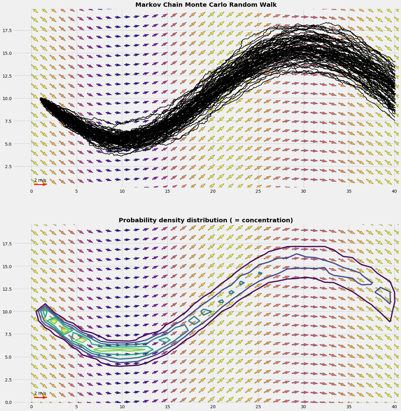
Example 1: Distribution in inhomogeneous conditions

We generate the mean drift data as an inhomogeneous flow field. It might be a water current in a river bed or an air flow in a valley. Usually fluid dynamics are modelled by the Navier Stokes equations. For sake of brevity we have generated the flow field by some analytical formula.

The random component represents the turbulence which is superimposed to the mean flow. Also for sake of brevity we simulate the turbulence by a singel constant value (standard deviation). So in the following example the turbulence field is homogeneous.

In this first example turbulence is small. We see a pattern as it can be expected from an air flow in cold nocturnal conditions.

#------ main: Mean Drift ----------        
nx,ny = 40, 20
X,Y,x,y,xc,yc = get_grid(nx,ny)
u,v = get_flowfield(X,Y,'C')

#------ main: Random Walk ----------   
nTraj, dt, sigma  = 80,  0.1,  0.6
xts,yts,C = run_randomWalk(nTraj,dt,sigma) 
plot_distribution(X,Y,u,v,xts,yts,xc,yc,C)

png

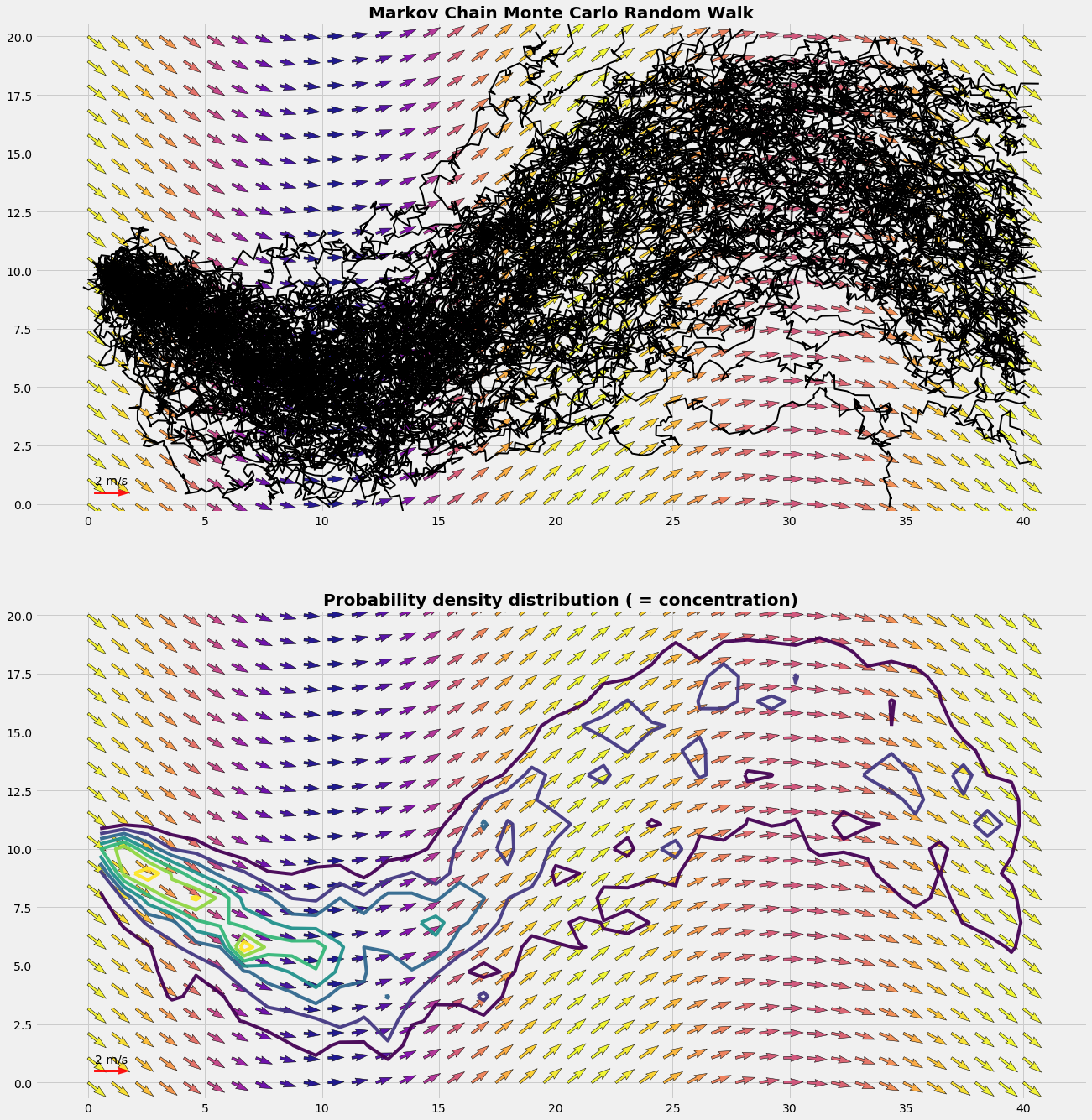
Example 2 : Distribution on a convective summer day

On a warm summer day turbulence is enhanced. The random component is now much more important relative to the same mean drift as in example 1. The sample particle gets each time step onto a different path of the mean drift.

#------ main: Random Walk ----------   
nTraj, dt, sigma  = 80,  0.1,  2.5
xts,yts,C = run_randomWalk(nTraj,dt,sigma) 
plot_distribution(X,Y,u,v,xts,yts,xc,yc,C)

png

Python code

import numpy as np
import pandas as pd
import matplotlib.pyplot as plt

def get_grid(nx,ny):
    x = np.linspace(0,nx,nx)
    y = np.linspace(0,ny,ny)
    X = np.outer(x,np.ones_like(y))  # X = ix.T * ones(iy)
    Y = np.outer(np.ones_like(x),y)  # Y = ones(ix) * iy.T
    xc = X + 0.5*(x[1]-x[0])
    yc = Y + 0.5*(y[1]-y[0])
    return X,Y,x,y,xc,yc

def get_flowfield(X,Y,case):
    if case == 'A': u,v = -Y, X
    if case == 'C':
        x =  2.0*np.pi*X/(np.amax(X)-np.amin(X)) +np.pi
        y =  0.5*np.pi*Y/(np.amax(Y)-np.amin(Y))
        u = 1 + 0.1*np.sin(x)
        v = 0.8*np.cos(x)
    return u,v

def inField(jx,jy):
    c = True
    if jx< 0: c=False; 
    if jx>nx: c=False
    if jy< 0: c=False; 
    if jy>ny: c=False
    return c

def fem4(ξ,ν):
    f1 = (1-ξ)*(1-ν); f2 = (ξ)*(1-ν)
    f3 = (ξ)*(ν);     f4 = (1-ξ)*(ν)
    return f1,f2,f3,f4

def get_V(xp,yp,jx,jy,u,v):
    ξ = (xp - x[jx])/(x[jx+1]-x[jx])
    ν = (yp - y[jy])/(y[jy+1]-y[jy])
    f1,f2,f3,f4 = fem4(ξ,ν)
    up = f1*u[jx,jy] + f2*u[jx+1,jy] + f3*u[jx+1,jy+1] + f4*u[jx,jy+1] 
    vp = f1*v[jx,jy] + f2*v[jx+1,jy] + f3*v[jx+1,jy+1] + f4*v[jx,jy+1]
    return up,vp

def get_cell(x,y,xp,yp, u,v, C):
    jx = np.argmax(x>=xp)-1
    jy = np.argmax(y>=yp)-1;
    if inField(jx,jy): 
        up,vp = get_V(xp,yp,jx,jy,u,v)
        C[jx,jy] += 1
        return up,vp,True
    else: 
        return [],[],False

def run_randomWalk(nTraj,dt,sigma):   
    xts = pd.DataFrame()
    yts = pd.DataFrame()
    C = np.zeros_like(xc)    
    for iTraj in np.arange(nTraj):
        xp = 1;  yp = y[0] + 0.5*(y[-1]-y[0])       
        xtr = np.array([xp])
        ytr = np.array([yp])
        while 1==1:
            up,vp,flag = get_cell(x,y,xp,yp,u,v, C)
            if flag:
                upp = np.random.normal(loc=0.0, scale=sigma) 
                vpp = np.random.normal(loc=0.0, scale=sigma) 
                xp = xp + (up+upp)*dt;  xtr = np.append(xtr, xp)
                yp = yp + (vp+vpp)*dt;  ytr = np.append(ytr, yp)
            else: 
                xts = pd.concat([xts,pd.DataFrame(xtr)], axis=1)
                yts = pd.concat([yts,pd.DataFrame(ytr)], axis=1)
                break
    return xts,yts,C

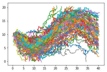
plt.plot(xts, yts); plt.show()

png

Grafics

def plot_flowfield(X,Y,u,v):
    R = (u*u + v*v)**(1/2)
    with plt.style.context('fivethirtyeight'): 
        fig = plt.figure(figsize=(15,15)) 
        ax1 = fig.add_subplot(111)
        q0 = ax1.quiver(X, Y, u, v, R, angles='xy', alpha=.92, cmap=plt.cm.plasma)
        q1 = ax1.quiver(X, Y, u, v, edgecolor='k', facecolor='None', linewidth=.5)
        p = plt.quiverkey(q0,1,0.5,2,"2 m/s",coordinates='data',color='r')
        ax1.set_aspect('equal')

def plot_trajectory(X,Y,u,v,xtr,ytr):
    R = (u*u + v*v)**(1/2)
    with plt.style.context('fivethirtyeight'): 
        fig = plt.figure(figsize=(15,15)) 
        ax1 = fig.add_subplot(111)
        q0 = ax1.quiver(X, Y, u, v, R, angles='xy', alpha=.92, cmap=plt.cm.plasma)
        q1 = ax1.quiver(X, Y, u, v, edgecolor='k', facecolor='None', linewidth=.5)
        p = plt.quiverkey(q0,1,0.5,2,"2 m/s",coordinates='data',color='r')
        ax1.plot(xtr,ytr,ls='-', color='k', lw=2, alpha=0.65)
        plt.title('Markov Chain Monte Carlo', fontsize=25, fontweight='bold')
        ax1.set_aspect('equal')

def plot_distribution(X,Y,u,v,xts,yts,xc,yc,C):
    R = (u*u + v*v)**(1/2)
    with plt.style.context('fivethirtyeight'): 
        fig = plt.figure(figsize=(20,22)) 

        ax1 = fig.add_subplot(211)
        q0 = ax1.quiver(X, Y, u, v, R, angles='xy', alpha=.92, cmap=plt.cm.plasma)
        q1 = ax1.quiver(X, Y, u, v, edgecolor='k', facecolor='None', linewidth=.5)
        p = plt.quiverkey(q0,1,0.5,2,"2 m/s",coordinates='data',color='r')        
        ax1.plot(xts,yts,'-k', lw=2)
        ax1.set_title('Markov Chain Monte Carlo Random Walk', fontsize=20, fontweight='bold')
        ax1.set_aspect('equal')

        ax2 = fig.add_subplot(212,sharex=ax1)
        q0 = ax2.quiver(X, Y, u, v, R, angles='xy', alpha=.92, cmap=plt.cm.plasma)
        q1 = ax2.quiver(X, Y, u, v, edgecolor='k', facecolor='None', linewidth=.5)
        p = plt.quiverkey(q0,1,0.5,2,"2 m/s",coordinates='data',color='r')
        ax2.contour(xc,yc, C ,  alpha=0.95)
        ax2.set_title('Probability density distribution ( = concentration)', fontsize=20, fontweight='bold')
        ax2.set_aspect('equal')

HealthyNumerics

Computational Fluid Dynamics: Markov Chain Monte Carlo in 2 dimensions