- Sa 27 Oktober 2018
- ComputationalFluidDynamics
- Peter Schuhmacher
- #flow model, #FVM, #curvilinear grid
Example
The mathematics of discretization
- is in detail given here
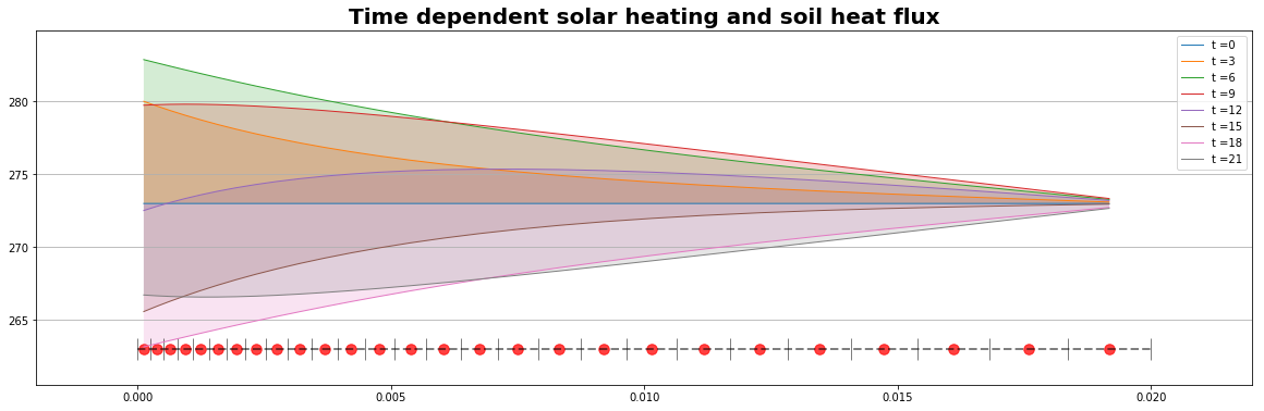
We solve the time dependent (= instationary) diffusion equation
- \(f(t)\) is the solar heating. It is time dependent according to the (relative) diurnal movement of the sun.
- the sun heats the ground and is the forcing term.
- \(T\) is the evolving (distribution of the) temperature.
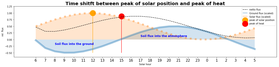
- during the morning hours there is a heat transport into the ground.
- But in the afternoon, when the solar force is declining, there is a heat flux from the ground into the atmosphere.
- The sum of the solar heating and the ground flux towards the atmosphere makes that the peak of the heat is in the afternoon and not at noon (when the sun is in the zenith).
Implicit (Euler backward) time schema
The implicit time schema the tendency term \(\mathbf{T}_t\) is discretizised as
The unknown quantity \(\mathbf{T}^{n}\) is on the left side of the equation including the equation system which has to be solved at each time step
The stencil for the implicit schema is now
Introducing \(\tilde{\mathbf{A}}\) we find the following form of discretisation:
Implementation
import numpy as np
import pandas as pd
import scipy.sparse as sps
from scipy.sparse.linalg import bicgstab
import matplotlib.pylab as plt

np.set_printoptions(linewidth=200, precision=3)
Signals
This are auxiliary functions to initialize the parameter values. We have prepared a collection of signals here
class signal:
    def scale(self,t):            return (t-t.min())/(t.max()-t.min())
    def add_noise(self,t):        return np.random.randn(t.shape[0])
    def line(self,t):             return self.scale(t)
    def uSignal(self,t):          return np.array(0.5*np.sign(t) + 0.5,dtype=int)
    def wSignal(self,t,dt):       return self.uSignal(t)-self.uSignal(t-dt)
    def expSignal(self,t):        return np.exp(t)
    def minus_exp_square(self,t): return np.exp(-t**2)
The FVM grid
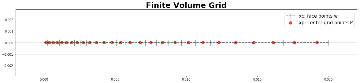
We generate a 1-dimensional grid with irregular spacing between the grid points. We start with the location of the faces and compute then the grid point in the center.
class grid1D:
    def __init__(self, nxc, Lx, sCase):
        self.nxc = nxc                                                         # number of faces
        self.Lx = Lx                                                           # length of x-domain
        sT = {'stretch_regular':self.stretch_regular,                          # mapping of stretching types
              'stretch_exp'    :self.stretch_exp}
        self.stretchT = sT[sCase]                                              # selects the type of stretching
    def scale(self, a):                    return (a-a.min())/(a.max()-a.min())# scaling to [0..1]
    def xi(self):                          return  np.linspace(0,1.0,self.nxc) # logical/computational grid
    def stretch_regular(self):             return  np.linspace(0,1.0,self.nxc) # regular grid, no stretching
    def stretch_exp(self):                                                     # exponantial stretching
        ix = self.xi();                    return  self.scale(np.exp(2*ix))
    def xc(self):                          return self.Lx*self.stretchT()      # face x-coordinate
    def xp(self):                          return self.centerPoint(self.xc())  # center point coordinate
    def dx(self):                                                              # spacing between P's
        xc = self.Lx*self.stretchT()
        x  = np.r_[xc[0],self.centerPoint(xc),xc[self.nxc-1]]
        return np.diff(x)
    def centerPoint(self,x): mx=x.shape[0]; return 0.5*(x[0:mx-1] + x[1:mx])    # center point P method
    def Swe(self):                          return np.ones((self.nxc))          # areas of the faces west-east
    def cvP(self):
        Swe = self.Swe(); mx=Swe.shape[0];
        return 0.5*(Swe[0:mx-1] + Swe[1:mx])*np.diff(self.xc())                 # volumes of the CV

#--- MAIN -------------------------------------------------------
#--- Input ------------------------------------------------------
nxc = 28                               # number of faces/corners
Lx  = 0.02                             # length of x-domain
#Lx  = 0.3                             # length of x-domain
nxp = nxc-1                            # number of central points P
#g  = grid1D(nxc,Lx,'stretch_regular') # 2 types
g   = grid1D(nxc,Lx,'stretch_exp')     # type of grid strechting
Graphics of the grid
#--- Graphics -----------------
#--- plot the grid ------------
xc = g.xc()                            # get the corners/faces points w, e
xp = g.xp()                            # get the central points P

def plot_grid(ax0,xc,xp, y_base=0):
    ax0.plot(xc, y_base+0*xc, c='k', ls='--', marker="|",ms=20, lw=2, alpha=0.5 )
    ax0.scatter(xp, y_base+0*xp,c='r', marker='o', s=90, alpha=0.75)
with plt.style.context('fast'):
    fig, ax0 = plt.subplots(figsize=(20,4))
    plot_grid(ax0,xc,xp)
    grid_legend = np.array(['xc: face points w', 'xp: center grid points P' ])
    plt.margins(0.1); plt.grid(axis='y'); plt.legend(grid_legend,prop={'size': 15})
    plt.title("Finite Volume Grid",fontsize=25, fontweight='bold')
    plt.show()
class system1D:
    def __init__(self,g,sig,case):
        self.g = g
        self.nxc = g.nxc
        self.nxp = self.nxc-1
        self.sig = sig
        self.case = case
    def b(self):        return np.zeros((self.nxp))             # initialize local rhs
    def DWE(self,g):    return self.gam()*g.Swe()/g.dx()        # build the non-zero elements of the system matrix
    #----- input section ------------------------------------------------------------------------------
    def T(self):
        if self.case=='B':   return 0.1*np.random.randn((self.nxp))  # initial value, random gauss [-0.1 .. +0.1]
        if self.case=='C':   return 273.0*np.ones((self.nxp))
    def q(self,g):
        if self.case=='B':   return 1000*(10**3) *g.cvP()       # set source term
        if self.case=='C':   return 0.00                        # set source term
    def gam(self):
        if self.case =='B':  return 0.5*np.ones((self.nxc))     # set diffusion coefficient
        if self.case =='C':  return 0.1*np.ones((self.nxc))     # set diffusion coefficient
    def T_west_fix(self):
         if self.case =='B': return 100.0                       # set T_fix at w-boundary
         if self.case =='C': return 273.0                       # set T_fix at w-boundary
    def T_east_fix(self):
         if self.case =='B': return 200.0                       # set T_fix at e-boundary
         if self.case =='C': return 273.0                       # set T_fix at e-boundary

def insert_boundary_conditions(sT,DWE,b):
    #----- input section ------------------------------------------------------------------------------
    west_fix = True  #---- west boundary                       # select type of boundary condition at w
    if west_fix:
        b[0] = sT.T_west_fix() * DWE[0];
    else: T_west_flux = 0; DWE[0] = T_west_flux

    east_fix = True   #---- east boundary                      # select type of boundary condition at e
    if east_fix:
        b[-1] =  sT.T_east_fix() * DWE[-1];
    else: DWE[-1] = 0.0
    return DWE,b
Time dependent algorithm
In this example the w-boundary oscillates with a sin-wave. The equations system has to be solved at each time step. After each time step the right hand side (RHS) has to be updated. It contains the solution of the previous time step.
def solve_timedependent_system(DWE,RHS,T,bT,ax0):
    def print_convergence(cc):
        if cc==0 : print("bicg-stab: successful exit --> c =",cc)
        if cc >0 : print("bicg-stab: convergence to tolerance not achieved, number of iterations is = ", cc)
        if cc <0 : print("bicg-stab: illegal input or breakdown --> c =",cc)

    #---- set integration time and time step
    tbegin, tend, dt = 0.0, 2*np.pi, 0.085*np.pi
    nTimeSteps = int( (tend-tbegin)/dt)+1;
    print('nTimeSteps', nTimeSteps)

    #---- center P ----
    DP =  1.0 - dt*(- DWE[0:nxp] - DWE[1:nxc]);
    #---- system matrix D ----
    DW =  -dt*DWE[1:nxp];   DE = -dt*DWE[1:nxp]
    D = sps.diags( diagonals=[DW, DP, DE],
                     offsets=[-1,  0,  1],
                     shape=(nxp, nxp), format='csr')

    #---- numerical solver -----
    Gflux= np.zeros((nTimeSteps))                # will evaluate the ground flux
    Sflux= np.zeros((nTimeSteps))                # will evaluate the 'solar' flux
    for jt in np.arange(nTimeSteps):             # the time loop
        t = jt*dt
        T_west_fix = 273 + 10.0*np.sin(t)        # update boundary value T[n]
        RHS     = T                              # update the RHS with T[n-1]
        RHS[0]  = dt*T_west_fix * DWE[0] + T[0]  # w BC: update the RHS with T[n-1]
        RHS[-1] = dt*bT[-1] + T[-1]              # e BC: update the RHS with T[n-1]

        X = bicgstab(D,RHS,x0=T,tol=1e-06, maxiter=None);
        T = X[0]
        Sflux[jt] = T_west_fix
        Gflux[jt] = -(T[0]-T[2])
        if jt%3 == 0:
            plt.plot(xp,T, marker='', lw=1.0, alpha=0.99,label='t ='+str(jt));
            plt.fill_between(xp,T,273.0, alpha=0.2)
    return T,Sflux,Gflux

#----- main --------------------
sig    = signal()                               # get access to the signals
sT     = system1D(g,sig,case='C')               # instantiate a system for this case
qT     = sT.q(g)                                # set the source term
#---- main ---------------------
DWE    = sT.DWE(g)                              # build the non-zero elements of the system matrix
bT     = sT.b()                                 # initialize the local rhs of this system
DWE,bT = insert_boundary_conditions(sT,DWE,bT)  # insert the boundary conditions: changes DWE and b
RHS    = bT+qT                                  # update the right hand side of the complete system
T      = sT.T()                                 # initialize T

#---- graphics ----------------------
with plt.style.context('fast'):
    fig, ax0 = plt.subplots(figsize=(20,6))
    plot_grid(ax0,xc,xp, y_base=263)
    #--- run the time-dependent solution ---------------------
    T,Sflux,Gflux = solve_timedependent_system(DWE,RHS,T,bT,ax0)

    plt.legend(prop={'size': 10})
    plt.margins(0.1); plt.grid(axis='y'); #plt.legend(prop={'size': 15})
    plt.title("Time dependent solar heating and soil heat flux",fontsize=20, fontweight='bold')
    plt.show()

with plt.style.context('fast'):
    mg = len(Gflux)
    tt =( 24*np.arange(mg)/mg)
    ti = np.round(np.r_[tt[6:],tt[0:6]]).astype(int)
    G = sig.scale(Gflux)-0.5
    S = sig.scale(Sflux)
    F = S+G
    sy = np.max(S); sx = 6;
    fy = np.max(F); fx = 9;

    fig, ax0 = plt.subplots(figsize=(20,4))
    plt.plot(tt,G, lw=8, alpha=0.4)
    plt.fill_between(tt,G,0, alpha=0.2,label='Ground flux (scaled)')

    plt.plot(tt,S, lw=8, ls=':', alpha=0.4)
    plt.fill_between(tt,S,0, alpha=0.2,label='Solar flux (scaled)')

    plt.plot(tt,F, 'k--', label='netto flux' )
    plt.scatter(sx,sy,c='orange', s= 600, label='peak of solar position')
    plt.scatter(fx,fy,c='red', s= 600, label='peak of heat')
    plt.vlines(sx,-0.5,sy,color='orange')
    plt.vlines(fx,-0.5,fy,color='red')

    plt.text(2,-0.2,'Soil flux into the ground', fontsize=12, fontweight='bold',color='b')
    plt.text(11,0.1,'Soil flux into the atmosphere', fontsize=12, fontweight='bold',color='b')
    plt.xticks(tt, ti, fontsize=15); plt.xlabel('Solar hour'),  plt.ylabel('rel. flux')
    plt.title("Time shitft between peak of solar position and peak of heat",fontsize=20, fontweight='bold')
    plt.legend();plt.margins(0.1);plt.show()
nTimeSteps 24